20 years of PyTables
Back in October 2002 the first version of PyTables was released. It was an attempt to store a large amount of tabular data while being able to provide a hierarchical structure around it. Here it is the first public announcement by me:
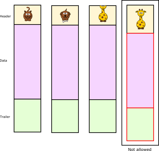
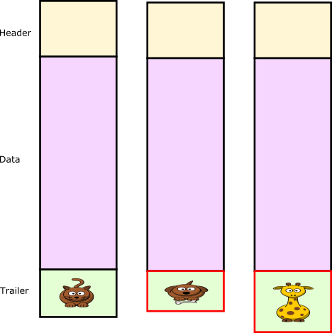
Hi!,

PyTables is a Python package which allows dealing with HDF5 tables.
Such a table is defined as a collection of records whose values are
stored in fixed-length fields.  PyTables is intended to be easy-to-use,
and tried to be a high-performance interface to HDF5.  To achieve this,
the newest improvements in Python 2.2 (like generators or slots and
metaclasses in brand-new classes) has been used.  Python creation
extension tool has been chosen to access the HDF5 library.

This package should be platform independent, but until now I’ve tested
it only with Linux.  It’s the first public release (v 0.1), and it is
in alpha state.
As noted, PyTables was an early adopter of generators and metaclasses that were introduced in the new (by that time) Python 2.2. It turned out that generators demonstrated to be an excellent tool in many libraries related with data science. Also, Pyrex adoption (which was released just a few months ago) greatly simplified the wrapping of native C libraries like HDF5.
By that time there were not that much Python libraries for persisting tabular data with a format that allowed on-the-flight compression, and that gave PyTables a chance to be considered as a good option. Some months later, PyCon 2003 accepted our first talk about PyTables. Since then, we (mainly me, with the support from Scott Prater on the documentation part) gave several presentations in different international conferences, like SciPy or EuroSciPy and its popularity skyrocketed somehow.
Cárabos Coop. V.
In 2005, and after receiving some good inputs on PyTables by some customers (including The HDF Group), we decided to try to make a life out of PyTables development and together with Vicent Mas and Ivan Vilata, we set out to create a cooperative called Cárabos Coop V. Unfortunately, and after 3 years of enthusiastic (and hard) work, we did not succeed in making the project profitable, and we had to close by 2008.
During this period we managed to make a professional version of PyTables that was using out-of core indexes (aka OPSI) as well as a GUI called ViTables. After closing Cárabos we open sourced both technologies, and we are happy to say that they are still in good use, most specially OPSI indexes, that are meant to perform fast queries in very large datasets; OPSI can still be used straight from pandas.
Crew renewal
After Cárabos closure, I (Francesc Alted) continued to maintain PyTables for a while, but in 2010 I expressed my desire to handover the project, and shortly after, a new gang of people, including Anthony Scopatz and Antonio Valentino, with Andrea Bedini joining shortly after, stepped ahead and took the challenge. This is where open source is strong: whenever a project faces difficulties, there are always people eager to jump up to the wagon and continue providing traction for it.
Attempt to merge with h5py
Meanwhile, the h5py package was receiving a great adoption, specially from the community that valued more the multidimensional arrays than the tabular side of the things. There was a feeling that we were duplicating efforts and by 2016, Andrea Bedini, with the help of Anthony Scopatz, organized a HackFest in Perth, Australia where developers of the h5py and PyTables gathered to attempt a merge of the two projects. After the initial work there, we continued this effort with a grant from NumFOCUS.
Unfortunately, the effort demonstrated to be rather complex, and we could not finish it properly (for the sake of curiosity, the attempt is still available). At any rate, we are actively encouraging people using both packages depending on the need; see for example, the tutorial on h5py/PyTables that Tom Kooij taught at SciPy 2017.
Satellite Projects: Blosc and numexpr
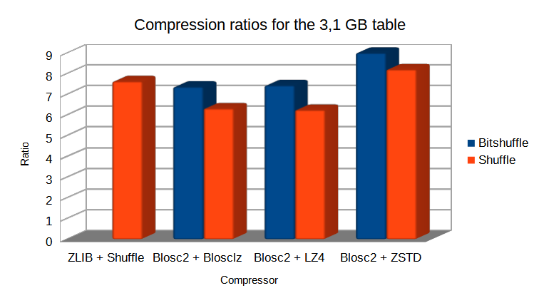
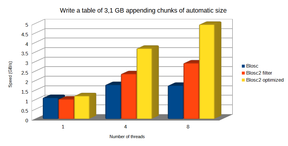
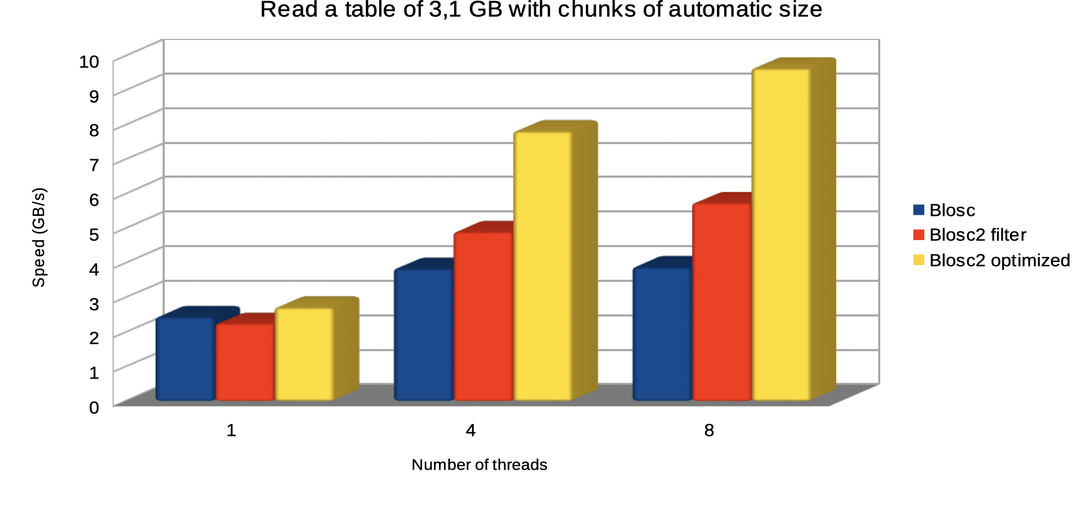
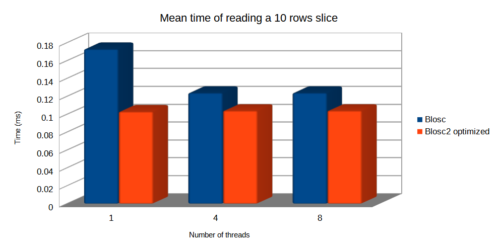
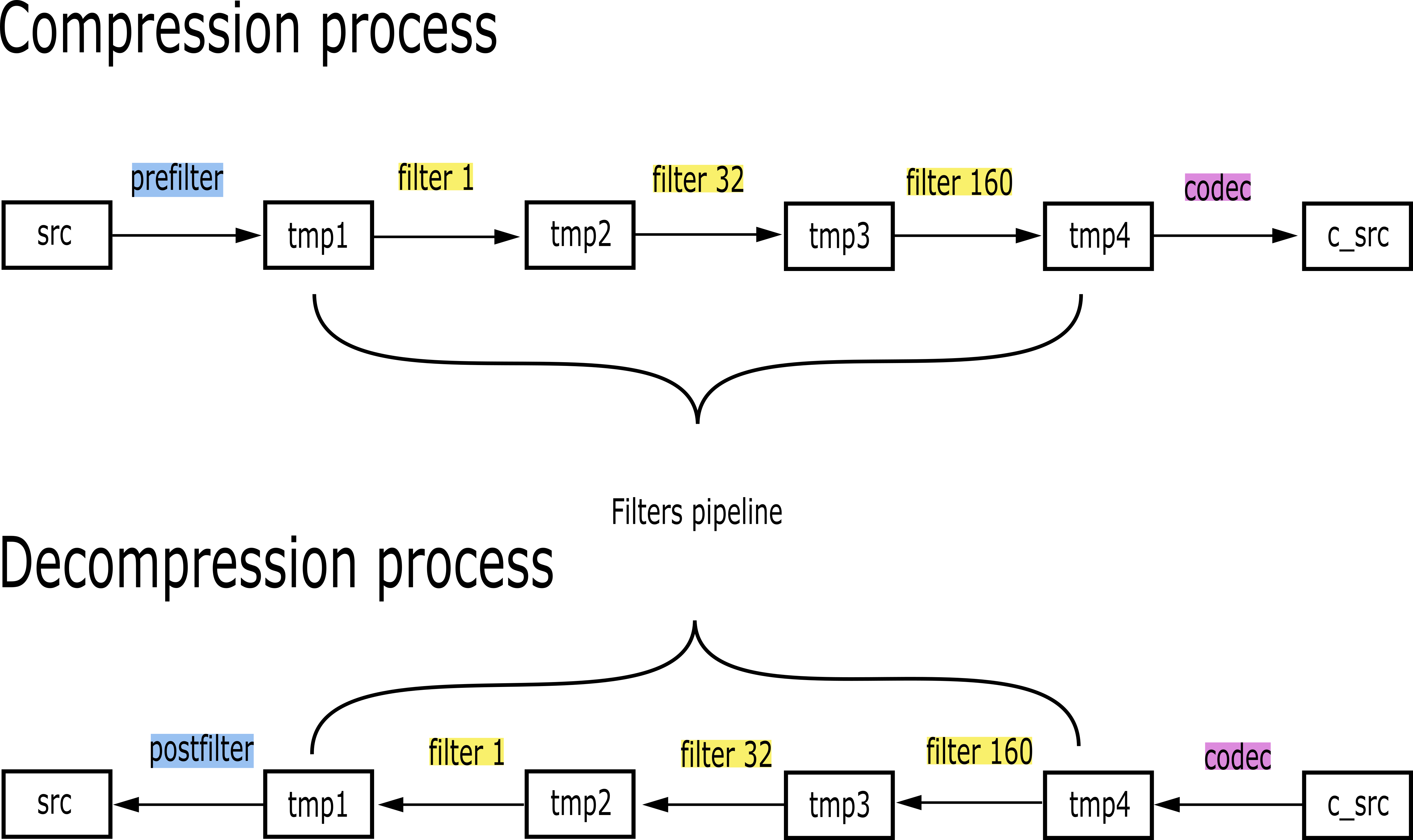
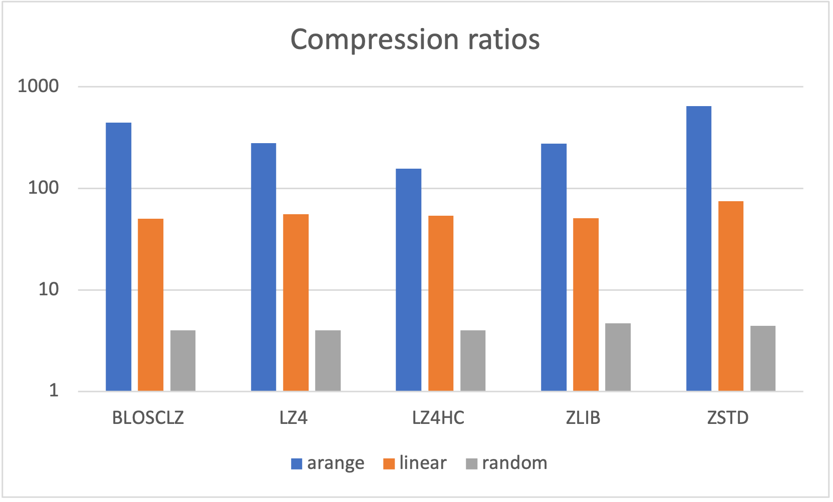
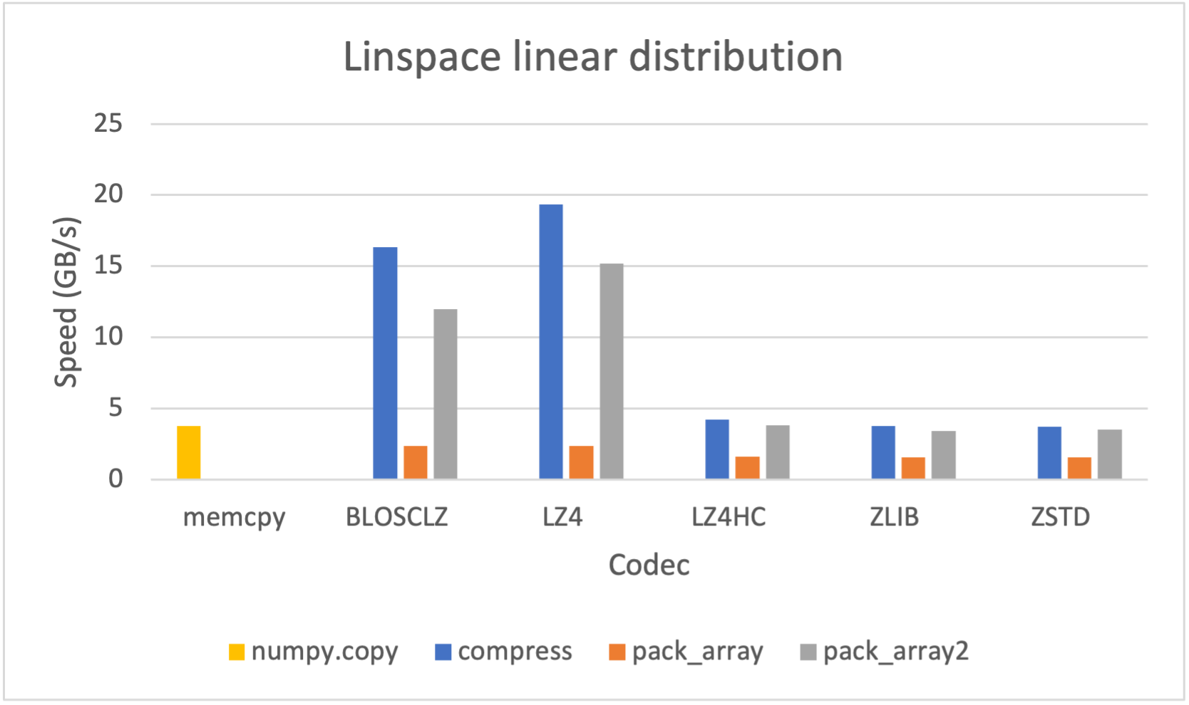
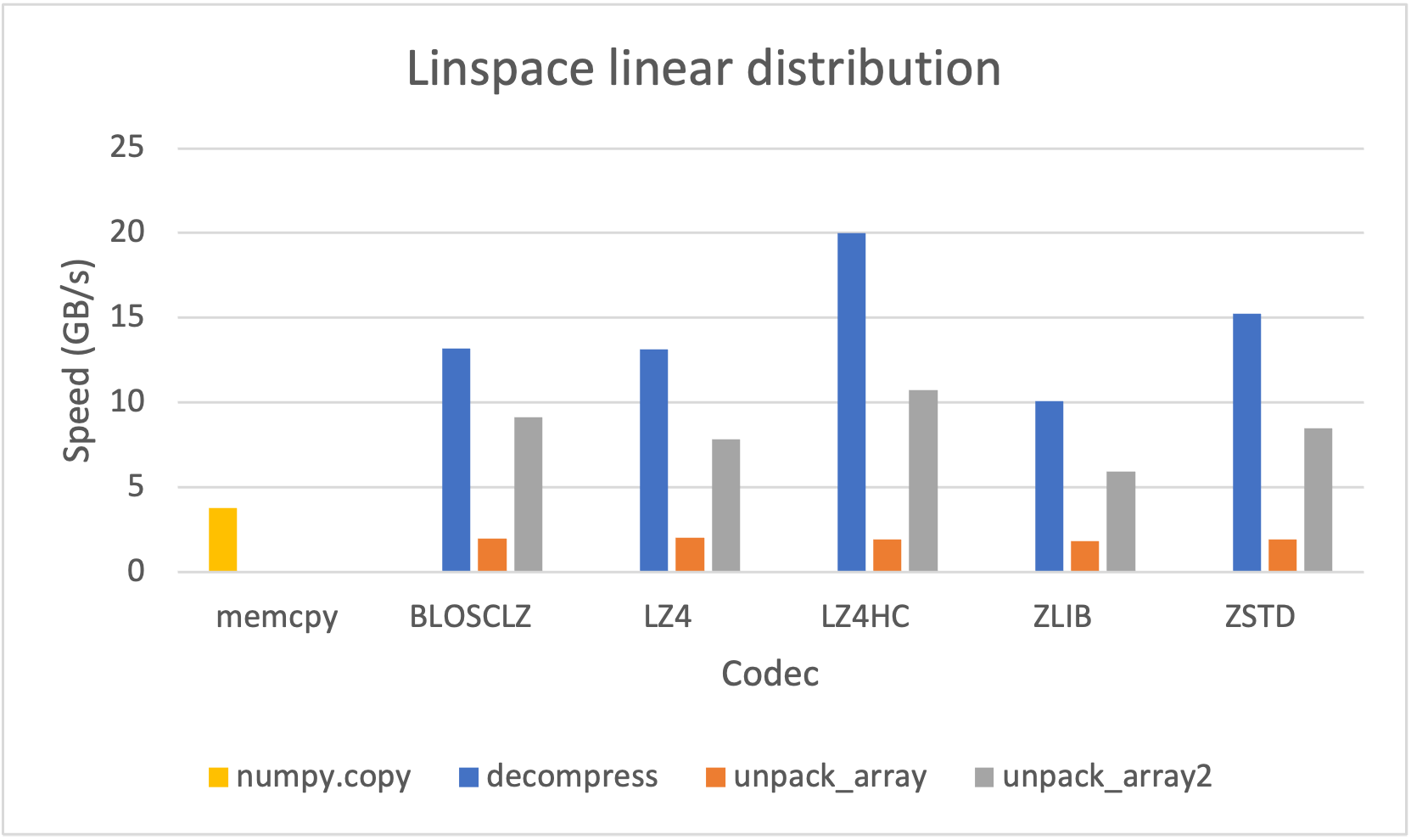
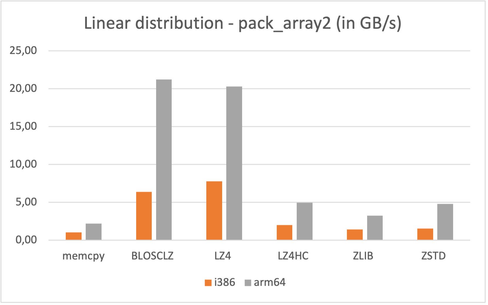
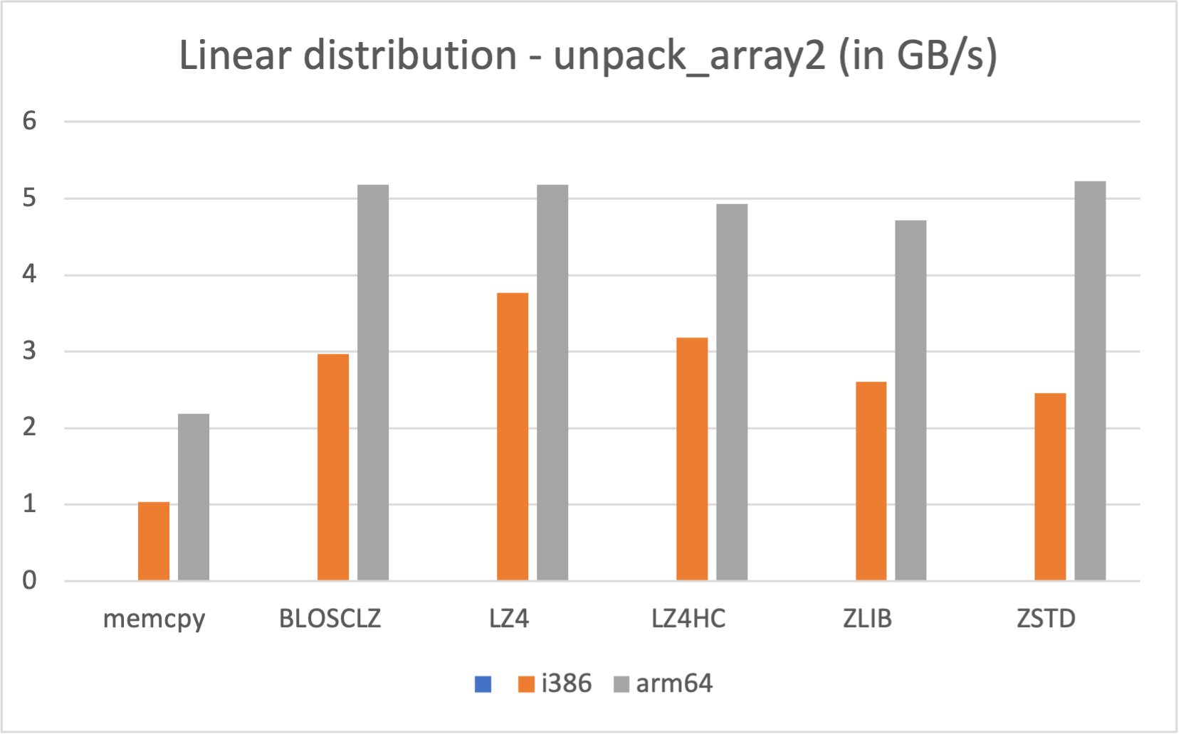
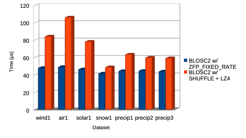
As many other open sources libraries, PyTables stands in the shoulders of giants, and makes use of amazing libraries like HDF5 or NumPy for doing its magic. In addition to that, and in order to allow PyTables push against the hardware I/O and computational limits, it leverages two high-performance packages: Blosc and numexpr. Blosc is in charge of compressing data efficiently and at very high speeds to overcome the limits imposed by the I/O subsystem, while numexpr allows to get maximum performance from computations in CPU when querying large tables. Both projects have been substantially improved by the PyTables crew, and actually, they are quite popular by themselves.
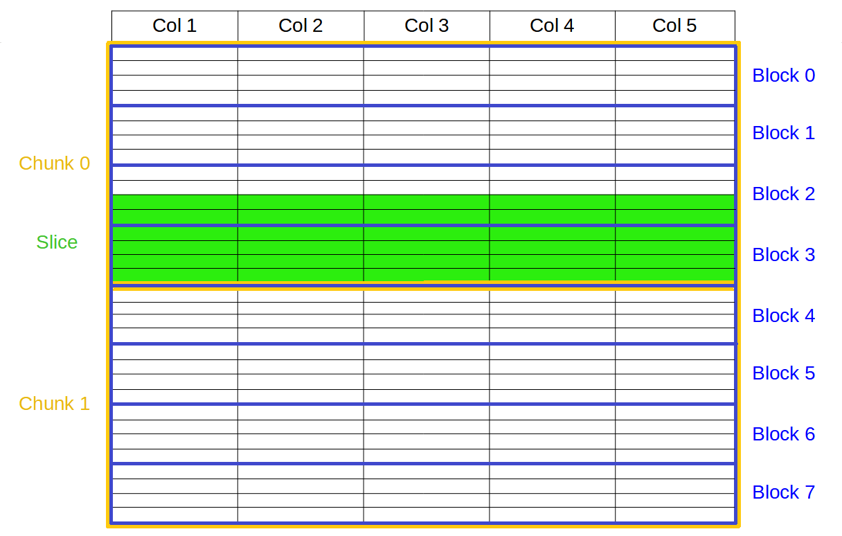
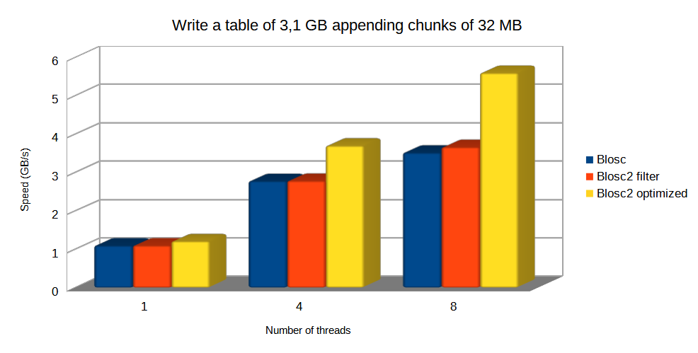
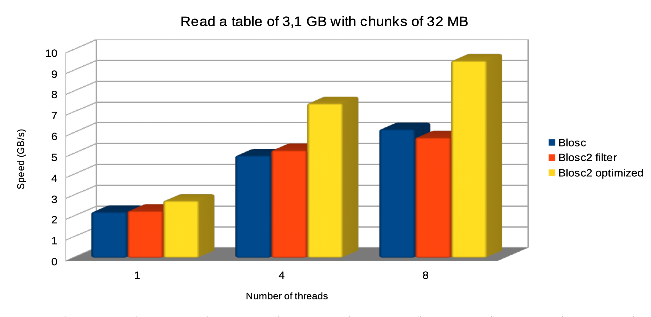
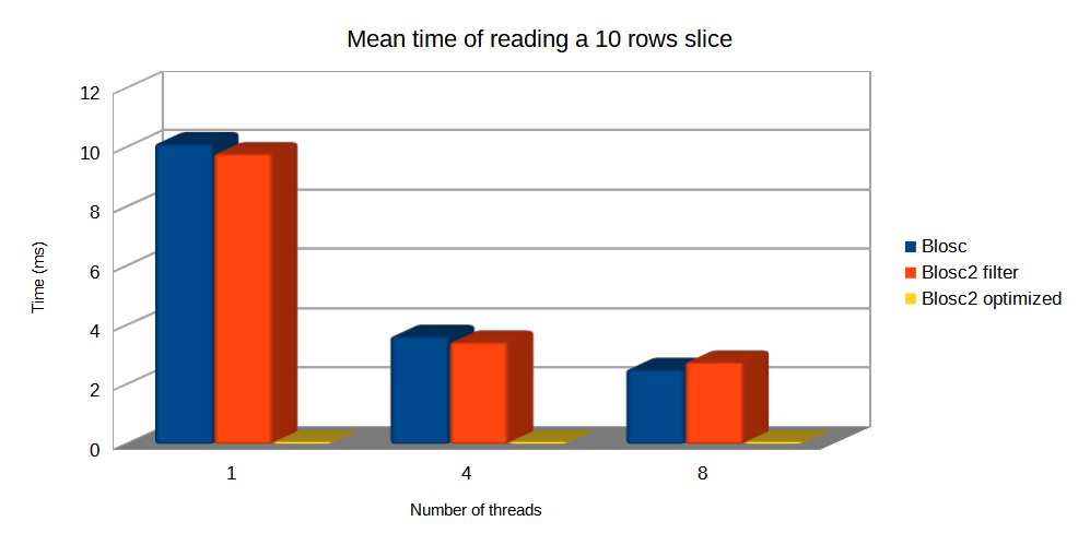
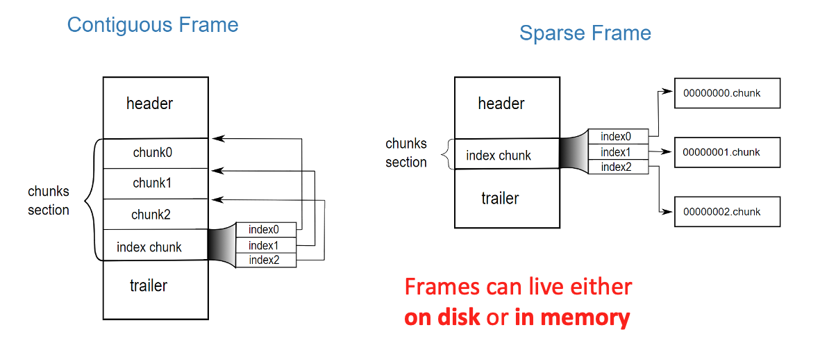
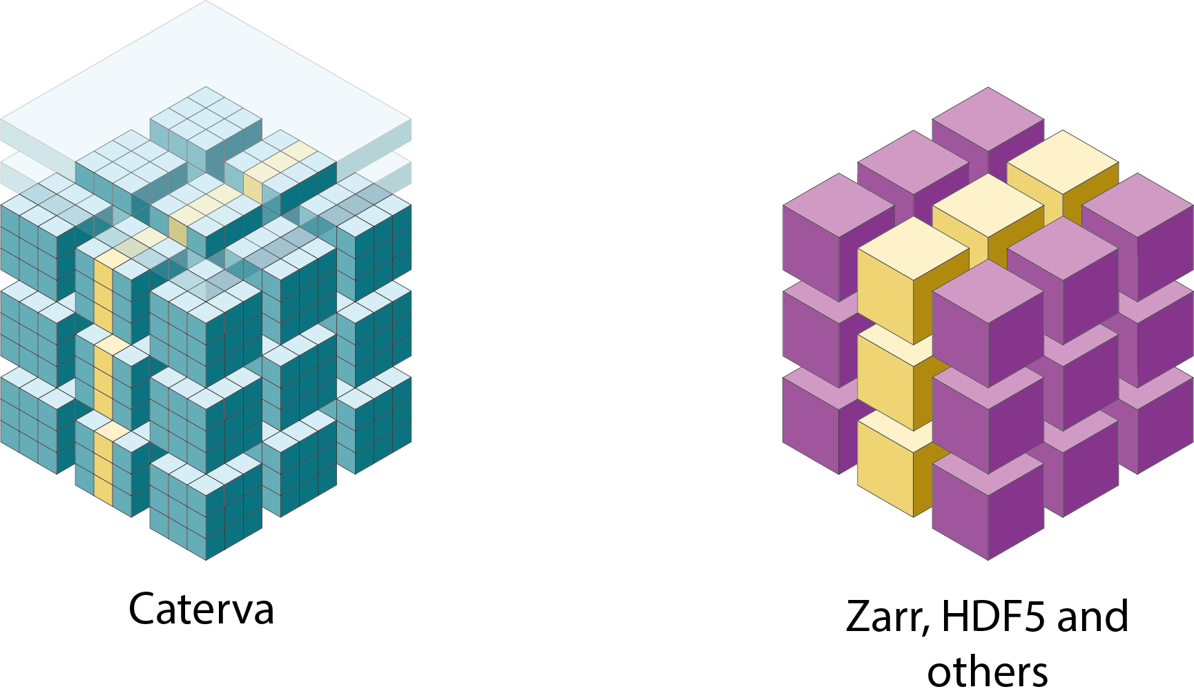
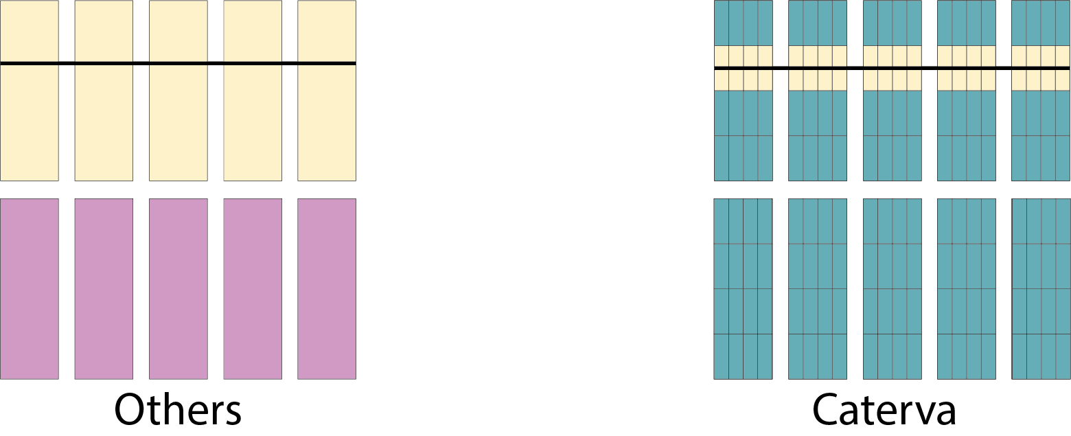
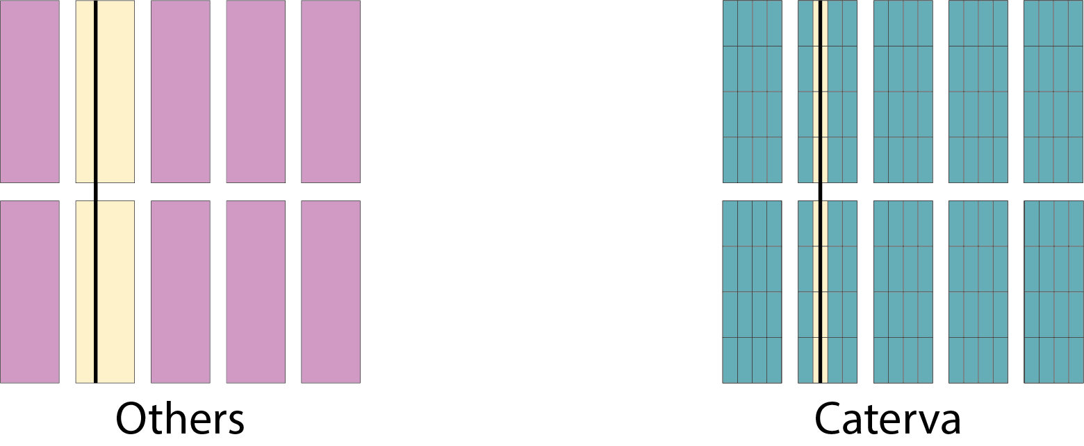
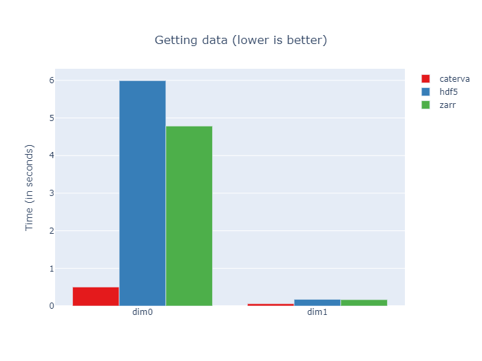
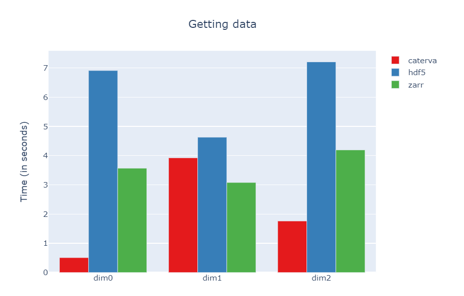
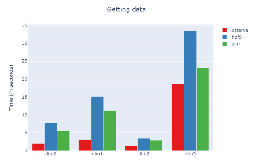
Specifically, the Blosc compressor, although born out of the needs of PyTables, it spun off as a standalone compressor (or meta-compressor, as it can use several codecs internally) meant to accelerate not just disk I/O, but also memory access in general. In an unexpected twist, Blosc2, has developed its own multi-level data partitioning system, which goes beyond the single-level partitions in HDF5, and is currently helping PyTables to reach new performance heights. By teaming with the HDF5 library (and hence PyTables), Blosc2 is allowing PyTables to query 100 trillion rows in human timeframes.
Thank you!
It has been a long way since PyTables started 20 years ago. We are happy to have helped in providing a useful framework for data storage and querying needs for many people during the journey.
Many thanks to all maintainers and contributors (either with code or donations) to the project; they are too numerous to mention them all here, but if you are reading this and are among them, you should be proud to have contributed to PyTables. In hindsight, the road may have been certainly bumpy, but it somehow worked and many difficulties have been surpassed; such is the magic and grace of Open Source!