Blosc2 Meets PyTables: Making HDF5 I/O Performance Awesome
PyTables lets users to easily handle data tables and array objects in a hierarchical structure. It also supports a variety of different data compression libraries through HDF5 filters. With the release of PyTables 3.8.0, the Blosc Development Team is pleased to announce the availability of Blosc2, acting not only as another HDF5 filter, but also as an additional partition tool (aka 'second partition') that complements the existing HDF5 chunking schema.
By providing support for a second partition in HDF5, the chunks (aka the 'first partition') can be made larger, ideally fitting in cache level 3 in modern CPUs (see below for advantages of this). Meanwhile, Blosc2 will use its internal blocks (aka the second partition) as the minimum amount of data that should be read and decompressed during data retrieval, no matter how small the hyperslice to be read is.
When Blosc2 is used to implement a second partition for data (referred ahead as 'optimized Blosc2' too), it can bypass the HDF5 pipeline for writing and for reading. This brings another degree of freedom when choosing the different internal I/O buffers, which can be of extraordinary importance in terms of performance and/or resource saving.
How second partition allows for Big Chunking
Blosc2 in PyTables is meant for compressing data in big chunks (typically in the range of level 3 caches in modern CPUs, that is, 10 ~ 1000 MB). This has some interesting advantages:
It allows to reduce the number of entries in the HDF5 hash table. This means less resource consumption in the HDF5 side, so PyTables can handle larger tables using less resources.
It speeds-up compression and decompression because multithreading works better with more blocks. Remember that you can specify the number of threads to use by using the MAX_BLOSC_THREADS parameter, or by using the BLOSC_NTHREADS environment variable.
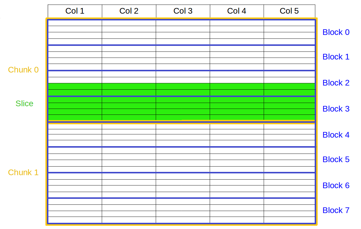
However, the traditional drawback of having large chunks is that getting small slices would take long time because the whole chunk has to be read completely and decompressed. Blosc2 surmounts that difficulty like this: it asks HDF5 where chunks start on-disk (via H5Dget_chunk_info()), and then it access to the internal blocks (aka the second partition) independently instead of having to decompress the entire chunk. This effectively avoids penalizing access to small data slices.
In the graphic below you can see the second partition in action where, in order to retrieve the green slice, only blocks 2 and 3 needs to be addressed and decompressed, instead of the (potentially much) larger chunk 0 and 1, which would be the case for the traditional 1 single partition in HDF5:
In the benchmarks below we are comparing the performance of existing filters inside PyTables (like Zlib or Blosc(1)) against Blosc2, both working as a filter or in optimized mode, that is, bypassing the HDF5 filter pipeline completely.
Benchmarks
The data used in this section have been fetched from ERA5 database (see downloading script), which provides hourly estimates of a large number of atmospheric, land and oceanic climate variables. To build the tables used for reading and writing operations, we have used five different ERA5 datasets with the same shape (100 x 720 x 1440) and the same variables (latitude, longitude and time). Then, we have built a table with a column for each variable and each dataset and added the latitude, longitude and time as columns (for a total of 8 cols). Finally, there have been written 100 x 720 x 1440 rows (more than 100 million) to this table, which makes for a total data size of 3.1 GB.
We present different scenarios when comparing resource usage for writing and reading between the Blosc and Blosc2 filters, including the Blosc2 optimized versions. First one is when PyTables is choosing the chunkshape automatically (the default); as Blosc2 is meant towards large chunks, PyTables has been tuned to produce far larger chunks for Blosc2 in this case (Blosc and other filters will remain using the same chunk sizes as usual). Second, we will visit the case where the chunkshape is equal for both Blosc and Blosc2. Spoiler alert: we will see how Blosc2 behaves well (and sometimes much beter) in both scenarios.
Automatic chunkshape
Inkernel searches
We start by performing inkernel queries where the chunkshape for the table is chosen automatically by the PyTables machinery (see query script here). This size is the same for Blosc, Zlib and uncompressed cases which are all using 16384 rows (about 512 KB), whereas for Blosc2 the computed chunkshape is quite larger: 1179648 rows (about 36 MB; this actually depends on the size of the L3 cache, which is automatically queried in real-time by PyTables and it turns out to be exactly 36 MB for our CPU, an Intel i9-13900K).
Now, we are going to analyze the memory and time usage of performing six inkernel searches, which means scanning the full table six times, in different cases:
With no compression; size is 3,1 GB.
Using HDF5 with ZLIB + Shuffle; size is 407 MB.
Using Blosc filter with BloscLZ codec + Bitshuffle; size is 468 MB.
Using Blosc2 filter with BloscLZ codec + Bitshuffle; size is 421 MB.
Using Blosc2 filter with Zstd codec + Bitshuffle; size is 341 MB.
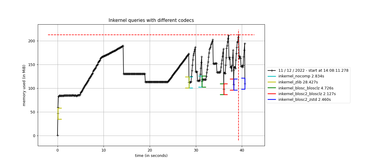
As we can see, the queries with no compression enable do not take much time or memory consumption, but it requires storing the full 3.1 GB of data. When using ZLIB, which is the HDF5 default, it does not require much memory either, but it takes a much more time (about 10x more), although the stored data is more than 6x smaller. When using Blosc, the time spent in (de-)compression is much less, but the queries still takes more time (1.7x more) than the no compression case; in addition, the compression ratio is quite close to the ZLIB case.
However, the big jump comes when using Blosc2 with BloscLZ and BitShuffle, since although it uses just a little bit more memory than Blosc (a consequence of using larger chunks), in exchange it is quite faster than the previous methods while achieving a noticeably better compression ratio. Actually, this combination is 1.3x faster than using no compression; this is one of the main features of Blosc (and even more with Blosc2): it can accelerate operation by using compression.
Finally, in case we want to improve compression further, Blosc2 can be used with the ZSTD codec, which achieves the best compression ratio here, in exchange for a slightly slower time (but still 1.15x faster than not using compression).
PyTables inkernel vs pandas queries
Now that we have seen how Blosc2 can help PyTables in getting great query performance, we are going to compare it against pandas queries; to make things more interesting, we will be using the same NumExpr engine in both PyTables (where it is used in inkernel queries) and pandas.
For this benchmark, we have been exploring the best configuration for speed, so we will be using 16 threads (for both Blosc2 and NumExpr) and the Shuffle filter instead of Bitshuffle; this leads to slightly less compression ratios (see below), but now the goal is getting full speed, not reducing storage (keep in mind that Pandas stores data in-memory without compression).
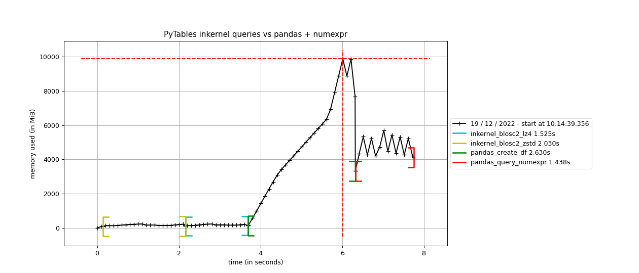
Here it is how PyTables and pandas behave when doing the same 6 queries than in the previous section.
And here it is another plot for the same queries, but comparing raw I/O performance for a variety of codecs and filters:
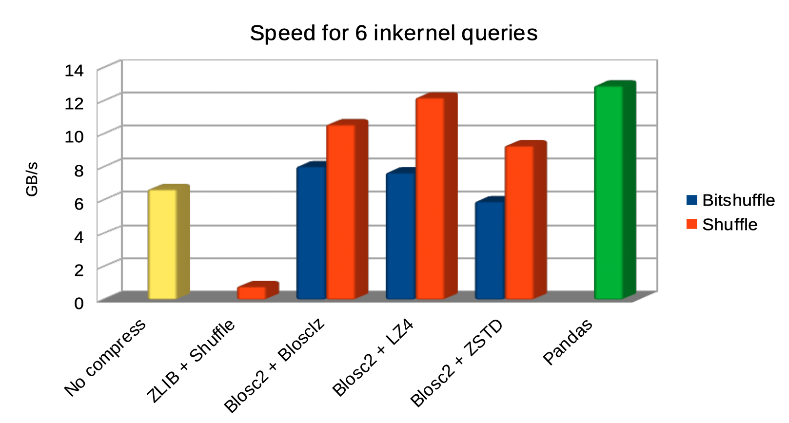
As we can see, the queries using Blosc2 are generally faster (up to 2x faster) than not using compression. Furthermore, Blosc2 + LZ4 get nearly as good times as pandas, while the memory consumption is much smaller with Blosc2 (as much as 20x less in this case; more for larger tables indeed). This is remarkable, as this means that Blosc2 compression results in acceleration that almost compensates for all the additional layers in PyTables (the disk subsystem and the HDF5 library itself).
And in case you wonder how much compression ratio we have lost by switching from Bitshuffle to Shuffle, not much actually:
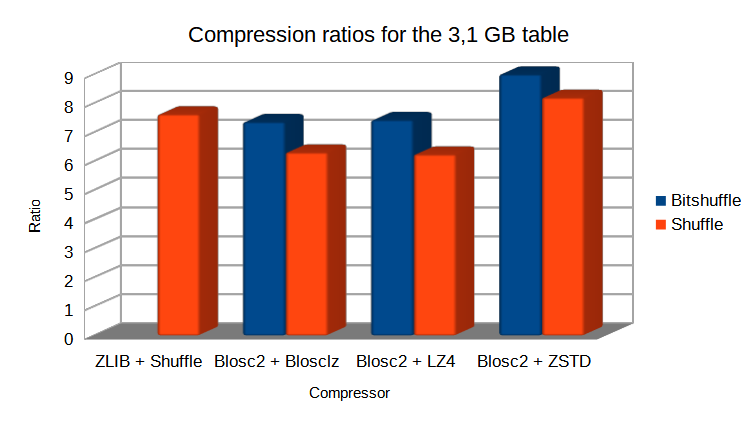
The take away message here is that, when used correctly, compression can make out-of-core queries go as fast as pure in-memory ones (even when using a high performance tool-set like pandas + NumExpr).
Writing and reading speed with automatic chunkshape
Now, let's have a look at the raw write and read performance. In this case we are going to compare Blosc, Blosc2 as an HDF5 filter, and the optimized Blosc2 (acting as a de facto second partition). Remember that in this section the chunkshape determination is still automatic and different for Blosc (16384 rows, about 512 KB) and Blosc2 (1179648 rows, about 36 MB).
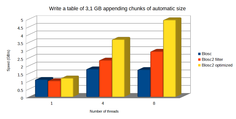
For writing, optimized Blosc2 is able to do the job faster and get better compression ratios than others, mainly because it uses the HDF5 direct chunking mechanism, bypassing the overhead of the HDF5 pipeline.
Note: the standard Blosc2 filter cannot make of use HDF5 direct chunking, but it still has an advantage when using bigger chunks because it allows for more threads working in parallel and hence, allowing improved parallel (de-)compression.
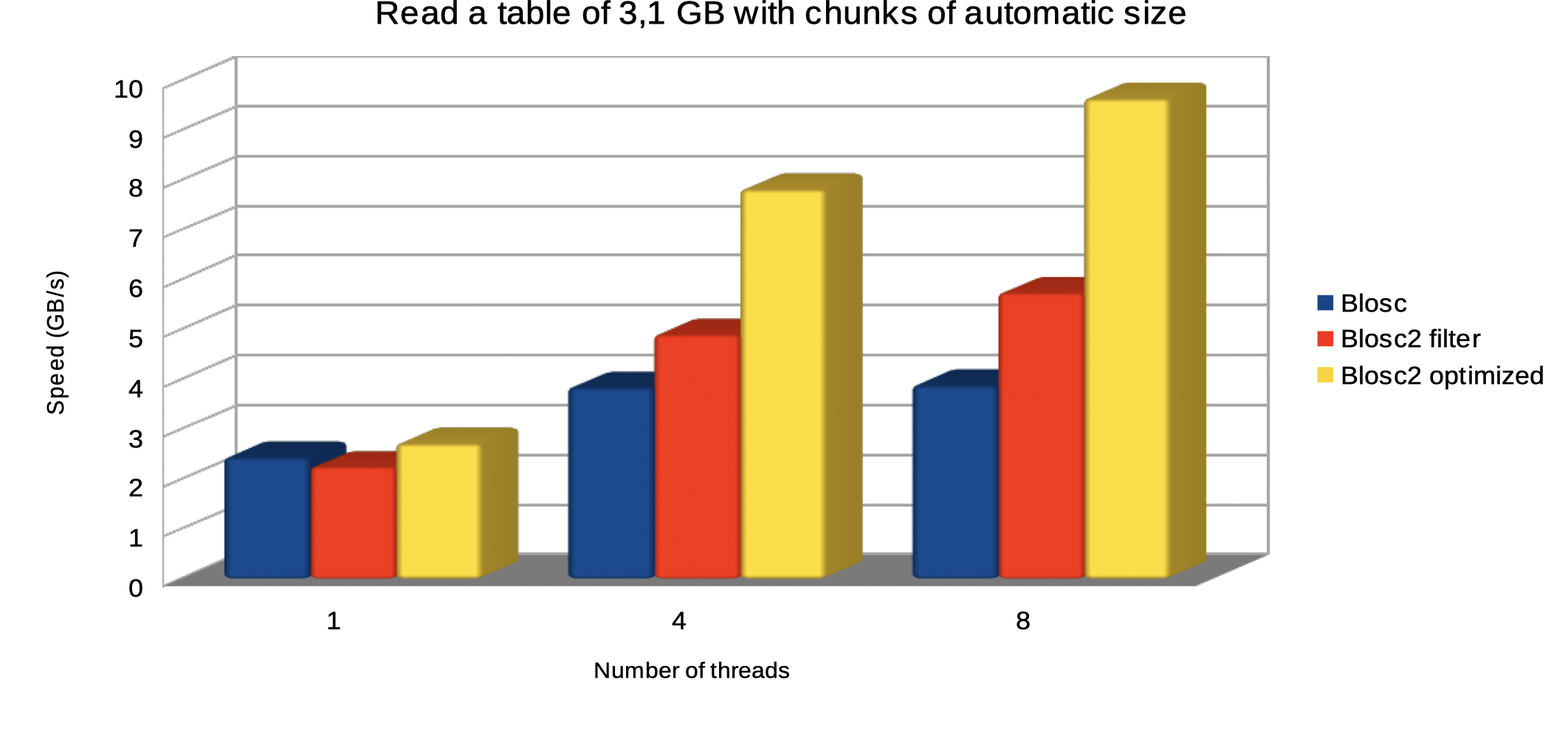
The plot below shows how optimized Blosc2 is able to read the table faster and how the performance advantage grows as we use more threads.
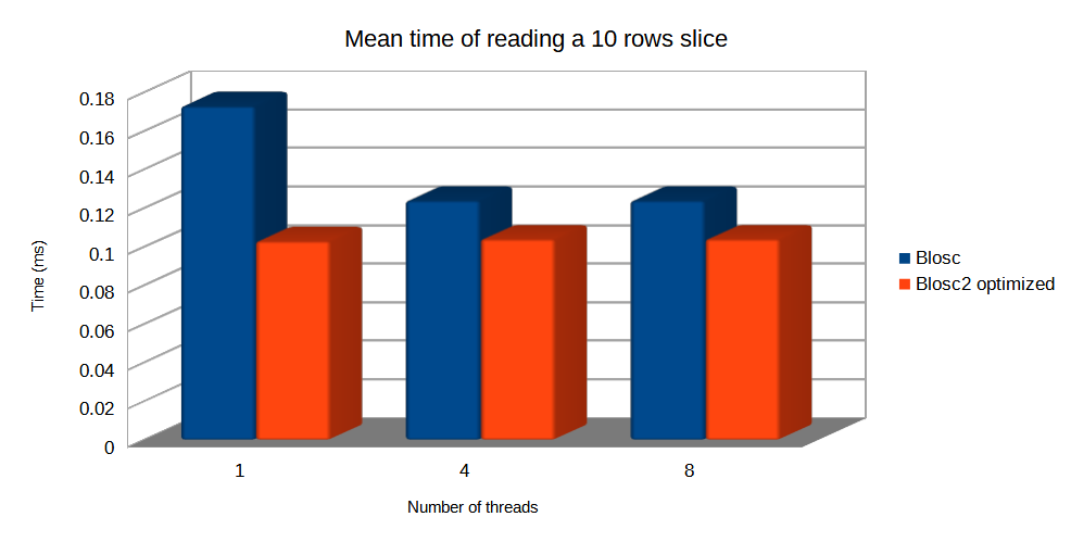
And now, let's compare the mean times of Blosc and Blosc2 optimized to read a small slice. In this case, Blosc chunkshape is much smaller, but optimized Blosc2 still can reach similar speed since it uses blocks that are similar in size to Blosc chunks.
Writing and reading speed when using the same chunkshape
In this scenario, we are choosing the same chunkshape (720 x 1440 rows, about 32 MB) for both Blosc and Blosc2. Let's see how this affects performance:
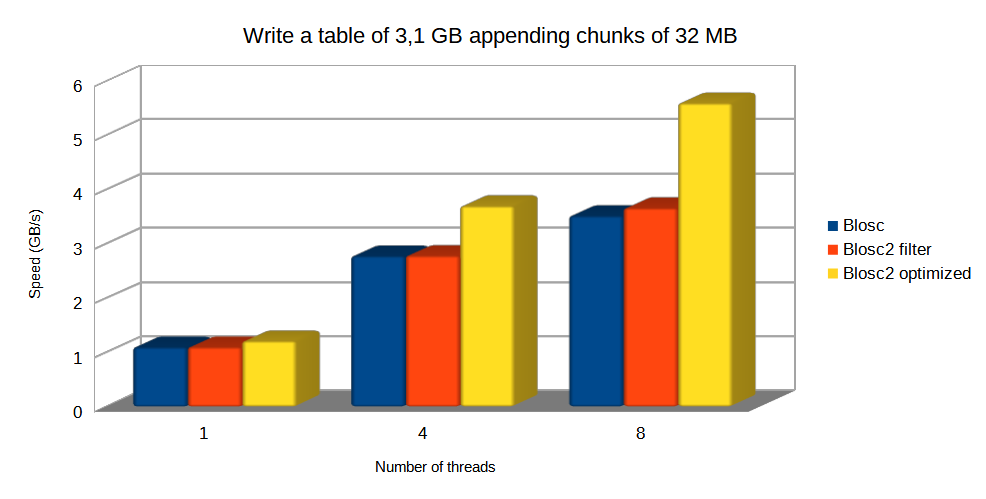
The plot above shows how optimized Blosc2 manages to write the table faster (mainly because it can bypass the HDF5 pipeline); with the advantage being larger as more threads are used.
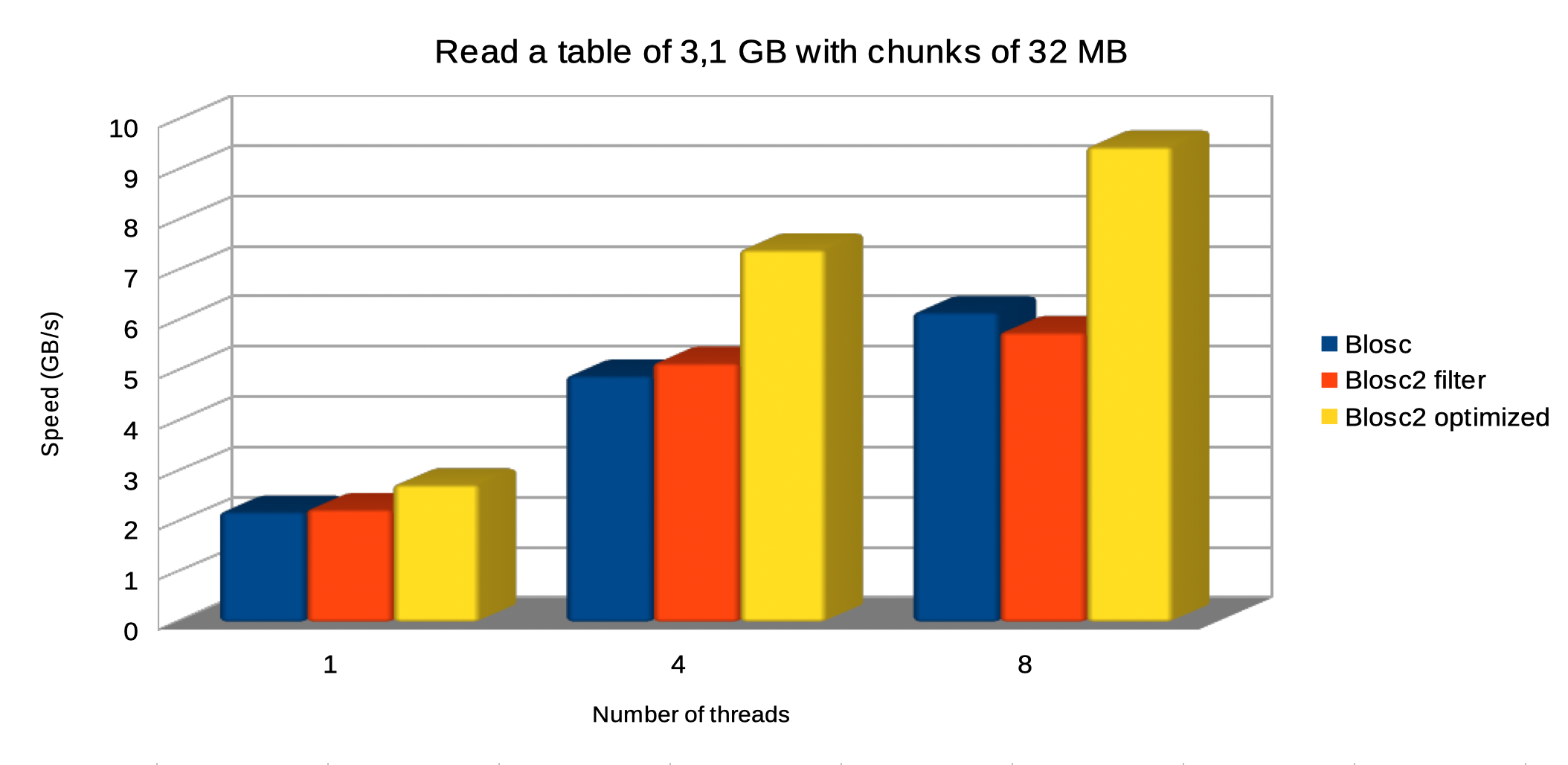
Regarding reading, the optimized Blosc2 is able to perform faster too, and we continue to see the same trend of getting more speed when more threads are thrown at the task, with optimized Blosc2 scaling better.
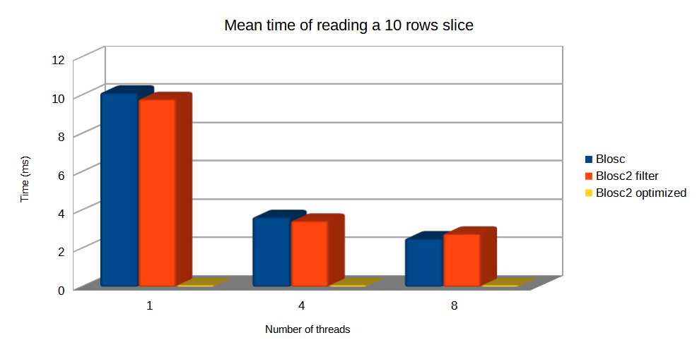
Finally, let's compare the mean times of Blosc and Blosc2 when reading a small slice in this same chunkshape scenario. In this case, since chunkshapes are equal and large, optimized Blosc2 is much faster than the others because it has the ability to decompresses just the necessary internal blocks, instead of the whole chunks. However, the Blosc and the Blosc2 filter still need to decompress the whole chunk, so getting much worse times. See this effect below:
Final words
By allowing a second partition on top of the HDF5 layer, Blosc2 provides a great boost in PyTables I/O speed, specially when using big chunks (mainly when they fit in L3 CPU cache). That means that you can read, write and query large compressed datasets in less time. Interestingly, Blosc2 compression can make these operations faster than when using no compression at all, and even being competitive against a pure in-memory solution like pandas (but consuming vastly less memory).
On the other hand, there are situations where using big chunks would not be acceptable. For example, when using other HDF5 apps that do not support the optimized paths for Blosc2 second partition, and one is forced to use the plain Blosc2 filter. In this case having large chunks would penalize the retrieval of small data slices too much. By the way, you can find a nice assortment of generic filters (including Blosc2) for HDF5 in the hdf5plugin library.
Also note that, in the current implementation we have just provided optimized Blosc2 paths for the Table object in PyTables. That makes sense because Table is probably the most used entity in PyTables. Other chunked objects in PyTables (like EArray or CArray) could be optimized with Blosc2 in the future too (although that would require providing a *multidimensional* second partition for Blosc2).
Last but not least, we would like to thank NumFOCUS and other PyTables donors for providing the funds required to implement Blosc2 support in PyTables. If you like what we are doing, and would like our effort to continue developing well, you can support our work by donating to PyTables project or Blosc project teams. Thank you!
Comments
Comments powered by Disqus