A compression library can go one of two ways: try to be everything (its own dataframe, its own query engine, its own format that nothing else reads), or be a fast, compact layer that slots underneath the tools you already use. Python-Blosc2 has initially leaned toward the first path, but this is changing quite dramatically. During the past year, we put a lot of effort in making Python-Blosc2 as much compatible as possible with the array API initiative.
And today's 4.9.1 release pushes compatibility with the tabular library ecosystem further than ever: CTable, our compressed table container, now plugs straight into Arrow, pandas, Polars and DuckDB.
Speaking Arrow
The star of this release is support for the Arrow PyCapsule protocol — the lingua franca of modern tabular tools. In plain terms: any Arrow-aware tool can now read a CTable directly, streaming it in small batches, without you converting anything first. Here is the same query — average fare per taxi company — asked five different ways, all against the same compressed file:
importblosc2t=blosc2.CTable.open("trips.b2z")# With Blosc2 itself...t.group_by("company").mean("fare")# ...or in SQL, with DuckDB reading the compressed table directlyimportduckdbduckdb.sql("SELECT company, avg(fare) FROM t GROUP BY company").show()# ...or with Polarsimportpolarsasplpl.DataFrame(t).group_by("company").agg(pl.col("fare").mean())# ...or with pandas >= 3.0importpandasaspdpd.DataFrame.from_arrow(t).groupby("company")["fare"].mean()# ...or with plain pyarrowimportpyarrowaspapa.table(t).group_by("company").aggregate([("fare","mean")])
Pick whichever syntax you like best — the data stays compressed on disk either way.
And it works the other way around too — hand CTable.from_arrow() a Polars dataframe, a pyarrow table or a Parquet reader, and you get a compressed table back:
Blosc2 isn't inventing anything here — it just implements a protocol the whole ecosystem already agreed on.
Strings that everyone understands
Text columns used to force an awkward choice in Blosc2: fixed-width strings (fast, but every value pays for the longest one) or variable-length strings (flexible, but slow to query). The new blosc2.utf8() column type ends that dilemma: it stores text in the exact same layout Arrow uses, so every row costs only what it needs — up to 13x less memory than fixed-width on free-form text — and data flows to and from Arrow tools with no translation.
And yes, it is fast: reading a full 10-million-row column requires just a fraction of a second; filtering is fast too, and utf8() even beats fixed-width strings as a group_by() key. Filters, sorting and grouping all work on it out of the box. However, sometimes you may still want to use string() / vlstring() for specific use cases; see the "Choosing a string column type" guide if you want the details.
Feeling at home for pandas users
CTable also picked up more of pandas' vocabulary this cycle, so familiar idioms now just work — chaining with assign() and col(), proper missing-data handling with fillna() and dropna(), and custom aggregation functions in group_by():
And if you'd rather stay in pandas entirely, you can still bring Blosc2's compute engine with you: df.apply(func, engine=blosc2.jit) now works correctly inside pandas 3, and Series.map() supports it too. See the "Using Blosc2 as a pandas engine" guide.
Cooperation, not completeness
Although CTable object comes with powerful machinery, it doesn't need to replace DuckDB, Polars or pandas to be useful; it just needs to hand them data in the shape they already expect — while doing the compression and fast querying underneath. If interoperating with the tools you already love sounds like the right job for a compression library, this is the release that makes the case.
Here is a question we have been chasing, in one form or another, for more than fifteen years: how much work can you avoid doing if your data is stored the right way?
In this post we put that question to a concrete test: one selective query against 24.3 million Chicago taxi trips, stored on disk in two formats — Parquet and the new persistent .b2z format for TreeStore and other Blosc2 objects — and answered by five different tools: DuckDB, PyArrow, pandas, polars, and Blosc2's own CTable. But let me first tell you how we got here, because CTable did not appear out of thin air: it is the fourth floor of a building whose foundations were laid in 2009.
From a turbo-charged compressor...
Blosc (acronym for BLOcked, Shuffled and Compressed) was born with a single, then-heretical idea: that compression could make data access faster, not slower. CPUs were (and are) starving — they can crunch numbers far faster than memory can feed them — so if you split data into blocks that fit in CPU caches, shuffle the bytes so that similar ones sit together, and decompress with all your cores, the time spent decompressing can be smaller than the time saved moving fewer bytes. "Compress faster than memcpy" was the provocative benchmark slogan of the time.
That first Blosc was humble: a blocked, multithreaded meta-compressor for binary buffers. No containers, no files, no types. Just speed.
...to containers, arrays, and a compute engine
The next decade taught us that a fast compressor alone is not enough; data needs a home. C-Blosc2 (2.0 released in 2021) gave it one: 64-bit super-chunks, persistent frames, a richer filter pipeline, modern codecs, and a plugin system. On the Python side, this matured into Python-Blosc2.
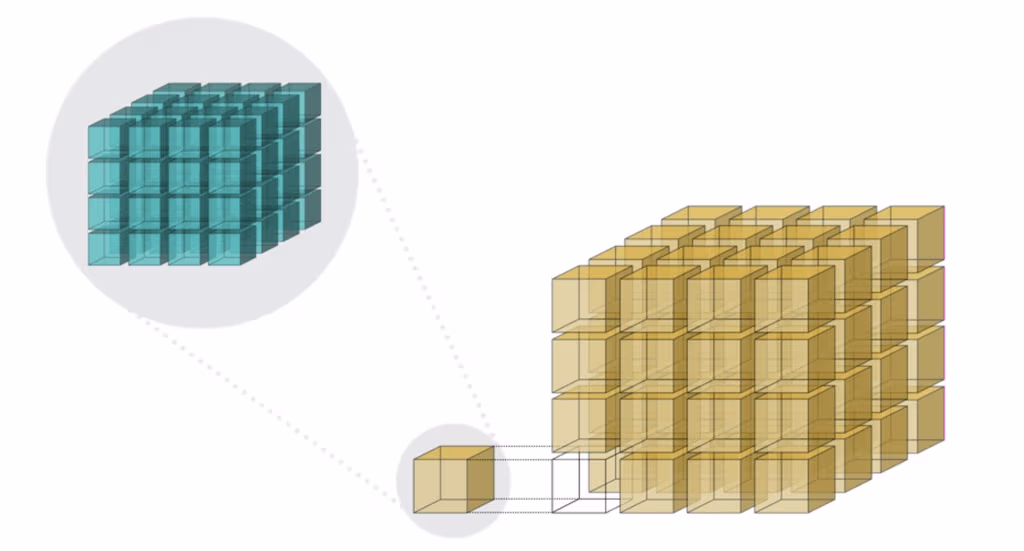
2023 came with both NDim and NDArray: a compressed, n-dimensional array, with a two-level partitioning scheme — chunks, sized to fit comfortably in higher-level CPU caches, divided into blocks — where the block is the unit of decompression, sized to fit comfortably in lower-level CPU caches. Slicing an NDArray decompresses only the blocks that the slice touches, and several blocks can be decompressed in parallel too (as long as they belong to the same chunk). Keep that sentence in mind; it is important for what comes below.
On top of that, Python-Blosc2 3.0 (early 2025) added a compute engine: lazy expressions like a + b * 2 that evaluate block by block, straight over compressed (possibly larger-than-RAM) operands, and return NumPy arrays. The engine never materializes whole arrays; it streams cache-sized blocks through the CPU. At this point we had fast compressed storage and fast compute over it — what we were missing was a way to talk about tables.
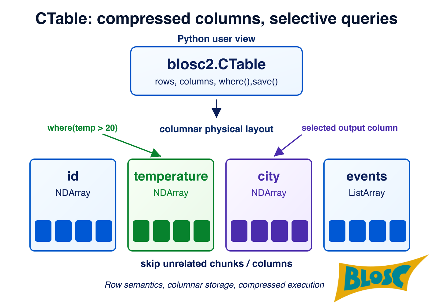
CTable: a columnar table on Blosc2 foundations
CTable (introduced in 2026) is exactly that: a columnar table where each column is an NDArray (or a ListArray for variable-length data), with typed schemas, nullable columns, and a where() method (among others) that accepts plain Python expressions and is executed by the compute engine.
Because columns are NDArrays, every column inherits the block structure — and this is where the design clicks together. CTable can build indexes for each column (like min/max statistics kept at block granularity). When a query like t.payment.tips > 100 arrives, blocks whose maximum tip is below 100 are never read and never decompressed. The index granularity is exactly aligned with the unit of work it avoids.
A CTable persists inside a .b2z file: the single-file, zip-based flavor of a persistent TreeStore that holds all columns, indexes and metadata in one compact, openable-anywhere container. Like Parquet, the data stays compressed on disk; unlike Parquet, you can open it and immediately get NumPy-addressable columns, no engine in between.
Now, where does the fourth floor hold the weight? Time to experiment.
The benchmark setup: one selective query, five tools
The dataset is the classic Chicago Taxi trips table, with a selection of 24.3 million rows, 14 columns (floats, timestamps, dictionary-encoded strings, and even a variable-length GPS path per trip). The query is a typical needle-in-a-haystack filter with projection and sort:
Only 67 of 24.3 million rows match — a highly selective query, which is precisely the regime where indexing can shine.
The contenders: DuckDB, PyArrow, pandas and polars querying the Parquet file, and Blosc2's CTable querying the .b2z. Every tool reads from disk on demand; nothing is preloaded. Each engine runs in a fresh subprocess, and it reports the query time each script measures internally, excluding interpreter and import overhead. Cold-cache runs happen right after flushing the OS file cache (sudo purge); warm runs are best-of-7. The machine is a Mac mini (Apple M4 Pro) with 24 GB RAM. The full, reproducible notebook is in the python-blosc2 repository.
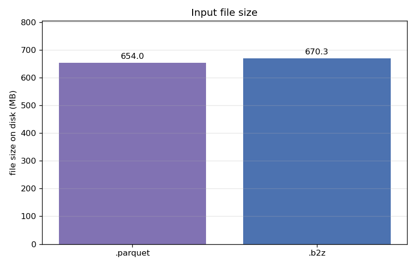
First, the storage footprint:
The .b2z lands at 670 MB versus Parquet's 654 MB — a 2% premium. Those extra bytes are mostly the block-level indexes. It is important to note that these indexes are computed automatically when importing a Parquet file into a CTable .b2z file.
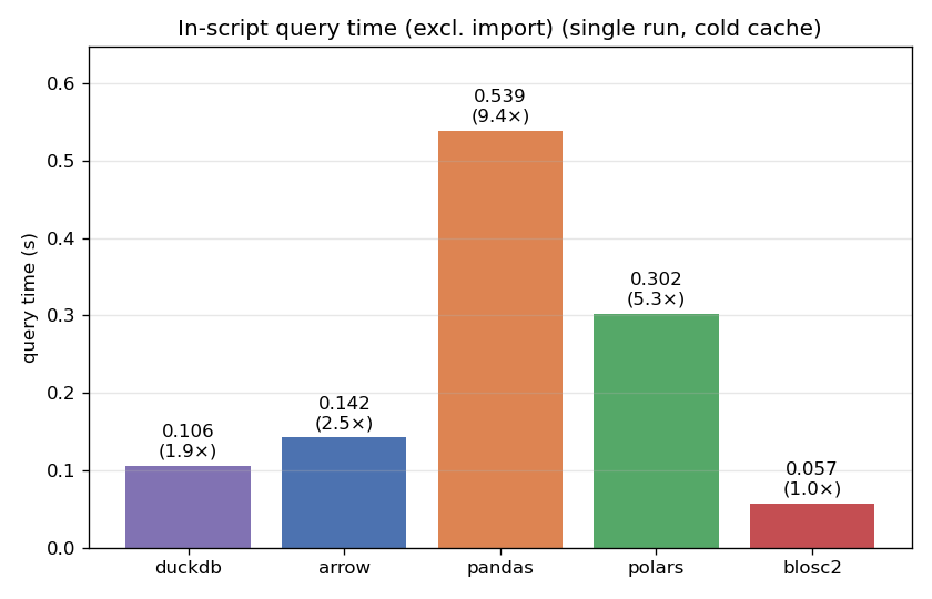
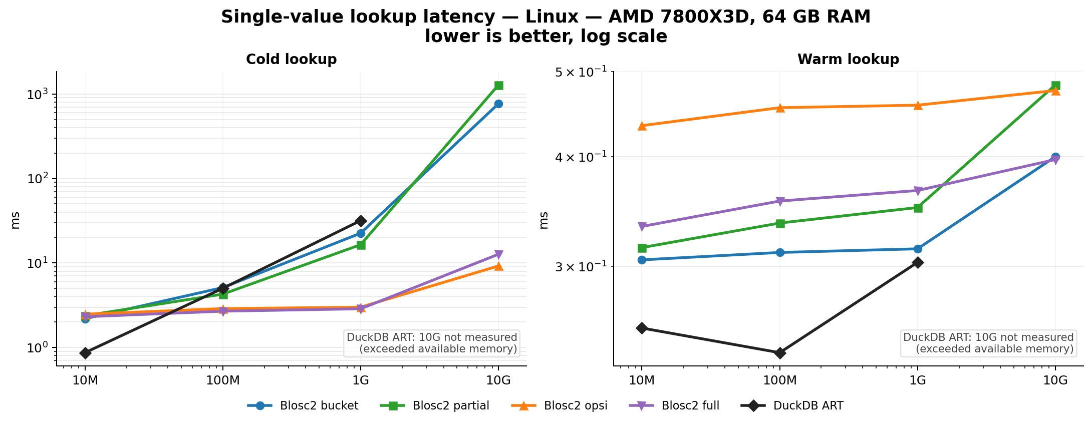
Cold cache: reading less wins
The cold run is the scenario we care most about: you have a large file on disk, it is not in the OS cache, and you want one answer, fast.
CTable answers in 0.057 s — about 1.9x faster than DuckDB (0.106 s), 2.5x faster than PyArrow, 5.3x faster than polars and 9.4x faster than pandas. It is important to note that all methods try to use streaming and filter pushdown where possible, although pandas is not designed for that, and it shows; interestingly polars is more advanced in that regard.
The reason why CTable can go faster is fine-grained indexing (min/max on blocks). On a cold cache, the dominant cost is bytes coming off the disk. The indexes let CTable prune roughly 90% of the blocks for this query: those blocks are neither read nor decompressed. Pruning pays twice — less I/O and less CPU — and on a first-touch query the I/O half is the whole ballgame. Parquet also has min/max statistics, but at a coarser row-group granularity, which for this query can prune nothing (see below).
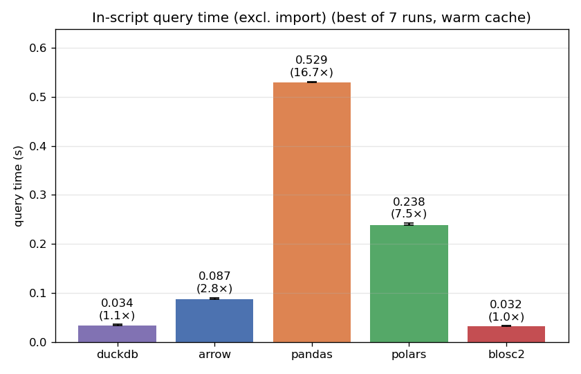
Warm cache: a dead heat with a real database
Once the file is fully cached in RAM, I/O is nearly free and raw engine throughput takes over. This is DuckDB's home turf — a vectorized, multithreaded analytical SQL engine with filter pushdown and late materialization.
CTable finishes in 0.032 s, DuckDB in 0.034 s — a dead heat (the two trade places within run-to-run noise), with both about 2.8x ahead of PyArrow, ~7x ahead of polars, and ~16x ahead of pandas. We find this result remarkable because Blosc2 brings no SQL engine: a storage container + compute + indexing engine holding the tie with a purpose-built database tells us the layout is doing the heavy lifting. Again, this layout is determined automatically, so users get the benefit without tuning.
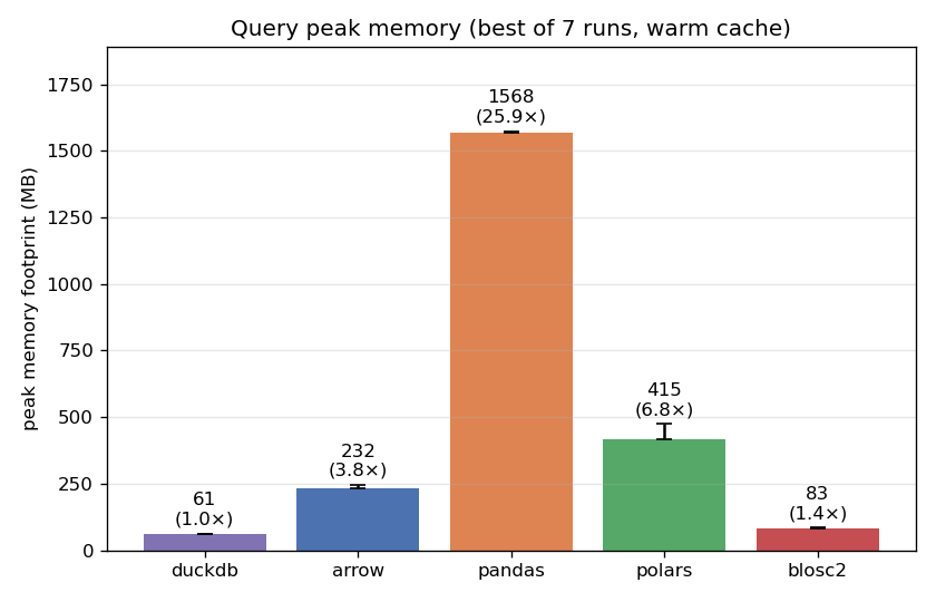
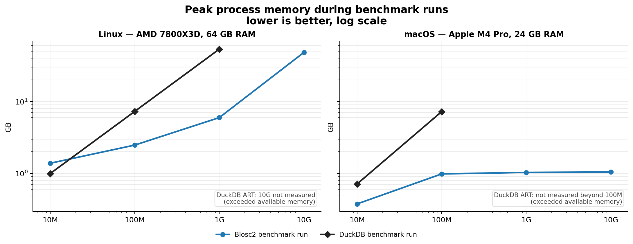
Memory tells a similar story:
DuckDB (~61 MB) and CTable (~83 MB) are the two leanest by a wide margin — more than an order of magnitude below pandas (~1.6 GB), which materializes full columns before filtering. polars can make use of better streaming, while PyArrow is still better, but both are still much heavier than the two leaders. This is important for large datasets that may not fit comfortably in RAM, because that means that larger-than-RAM queries are more likely to succeed without hitting swap when using CTable or DuckDB.
Why pruning wins: granularity
Parquet also carries min/max statistics — at row-group granularity, here ~970,000 rows per group. CTable keeps them at block granularity, ~27,000 rows per block: roughly 36x finer. A Blosc2 block is the unit of decompression — the same cache-sized block the compute engine streams. An index at a coarser granularity than the I/O unit can only skip work in big, lucky lumps. Choosing an appropriate block size is important, and this is automatically handled by Blosc2 when importing from Parquet.
Note that the advantage of indexes rides on selectivity, not on any general superiority. tips > 100 is rare enough that most 27K-row blocks contain no match.
Conclusions
Several interesting takeaways emerge from this experiment:
For selective cold queries on large tabular files, CTable/.b2z is genuinely fast — the fastest of the five tools here, on a query and dataset it was not specially tuned for. If your workload looks like "open a big file, fetch a small subset, move on", the block-level indexing earns its 2% of disk many times over.
Warm, it ties. DuckDB remains an excellent engine, and on cached data it matches CTable while speaking full SQL with joins and aggregations that CTable cannot cover (at least not yet). If your problems are relational, use a relational engine.
The result is arrays, not a result set.t.where(...) hands back NumPy-addressable columns with their original dtypes — no .to_numpy() hop, no DataFrame conversion tax. For NumPy-centric pipelines, that removes a whole impedance layer. And since columns are NDArrays, a CTable column can even be n-dimensional, or hold variable-length data (this dataset stores a GPS trace per row).
Parquet is not going anywhere. It remains the lingua franca of the data ecosystem, readable by everything. .b2z is young and its natural habitat is the Python/NumPy world. What this experiment shows is that the trade is real and the price is modest: a couple percent of disk for first-touch queries that run in a fraction of the time.
Sixteen years after asking whether compression could be faster than memcpy, the question has scaled up but taken on a slightly different shape: the fastest byte is the one you never touch. Blocks sized for caches made decompression cheap; the compute engine made math over blocks cheap; and CTable's block-level indexes now make not touching most of a table cheap, too. The fourth floor stands on the three below it.
Reproduce it yourself
Everything in this post lives in bench/chicago-taxi. The notebook, the driver, the five per-engine query scripts, and a README with the details. The notebook downloads the dataset on first run and builds the .b2z from it, so the whole thing is two commands away:
pip install "blosc2>=4.4.3" pyarrow duckdb polars pandas matplotlib jupyterjupyter-lab compare-query-methods.ipynb # then: Run All
The benchmark uses the Taxi Trips dataset published by the City of Chicago under its open data program. Thanks also to the NumFOCUS foundation and our sponsors for making sustained work on Blosc possible.
Working with large structured datasets in Python often means choosing between speed and simplicity. The new CTable object has born out of the need for a columnar store that compresses data on the fly, stays close to NumPy, and does not require an external database engine. It is the logical extension of current compressed data storage and computation in Python-Blosc2, brought to tabular datasets.
As compression is paramount in Blosc2 ecosystem, we have chosen a columnar approach because, by placing together data that is similar (values in the same column), it allows for best compression ratios. Column storage also allows for better data management for some cases, like adding, deleting, accessing or replacing entire columns; admittedly, it it also has its own drawbacks, like more costly access along the row axis. Nevertheless, columnar storage is quite common in modern libraries.
Another important piece for CTable is to leverage the extremely efficient compute engine that can operate on compressed data without dropping too much performance (and in some cases, even improving it). That puts the basis for allowing great analytics machinery on top of the CTable object, without the need to decompress entire columns (just small excerpts of them, fitting in CPU caches, is enough).
Last but not least, the CTable object inherits the independence of media storage of underlying structures (NDArray, ObjectArray, ListArray...) so that data can be stored and used straight from memory, disk or the network (coming soon). That means that you can open a data file containing a big CTable and immediately start doing analytics with it without the need to load/parse everything in-memory. Of course, for maximum speed, you may also load everything in-memory too; but as the format is the same, loading/saving is just a matter of copying data from one media to another, without the need for parsing or conversion.
Keep reading to learn more about CTable, its features and how to use it in your projects.
How it works
CTable stores each column as an independent blosc2.NDArray, compressed in chunks. Column types are defined through a schema — a plain Python dataclass where each field is annotated with a Blosc2 type spec such as b2.int64(), b2.float32(ge=0), or b2.string(). Specs can carry constraints (e.g. ge=0 for non-negative values) and are compiled into a schema that validates every row on insert, either one at a time via Pydantic or in bulk via vectorized NumPy checks.
Rows are tracked with a boolean tombstone mask: deleting a row simply flips its entry in the mask to False, with no data movement at all. The actual space is reclaimed lazily when you call compact(). Appending is also efficient because the underlying arrays are pre-allocated up front — they only grow when the pre-allocated capacity is exhausted, so there is no resize on every single insert.
Because the data lives in Blosc2 chunks, many queries can skip full chunks entirely. When a chunk's stored metadata (min/max) rules out any match, it is never decompressed. This is where a lot of the query speed comes from, and it is also why explicit indexes (described in Features below) can push performance even further.
Since blosc2.NDArray stores fixed-width binary data, null has no natural representation for integers, floats, or booleans. CTable solves this by letting you declare a column as nullable, and a sentinel value as the null marker is chosen automatically, although you can always use your own. For example, if you are storing ages and sometimes the value is unknown, you can set -1 as the null value since ages are never negative. Aggregates such as .mean() or .std() skip those rows automatically, and helper methods like .is_null() and .null_count() make it easy to work with them.
Not all data fits neatly into fixed-width columns though. Think of a column storing the tags of an article, the purchase history of a user, or the list of measurements taken at a sensor in a given day — each row may have a different number of items. For these cases CTable supports list columns, declared as blosc2.list(item_spec) (e.g. blosc2.list(blosc2.float32())), structured objects via blosc2.struct(item_spec) or completely general objects via b2.object(). These columns are backed by a different storage class internally, one that keeps a compressed stream of items alongside an offsets array to know where each row starts and ends. From the user's perspective they behave like any other column, but each cell holds a Python list instead of a scalar, and individual lists can also be None. Internally, the underlying C-Blosc2 has been improved (and released as 3.0.0) to allow variable-length data in super-chunks in a very efficient (and backward-compatible) way.
Main features
Creation: A CTable can be created in several ways. The most direct is declaring a typed schema as a dataclass and passing it to the constructor. You can also build a CTable from existing data — from_arrow() and from_csv() import Arrow tables and CSV files respectively, inferring or mapping types automatically. Finally, copy() produces a new independent CTable from an existing one, already compacted.
Modification: Appending a single row uses append(), while bulk insertion uses extend(). Deleting rows sets their mask entry to False and is essentially free. Columns can be added with a default value or dropped and renamed at any time. Beyond stored columns, CTable also supports two kinds
of virtual columns: computed columns are evaluated on-the-fly from an expression over other columns and never touch storage; materialized columns look like stored columns but are auto-filled automatically during every extend().
Querying: where(expr) filters rows and returns a view — a new CTable object that shares the same column arrays as the parent but carries its own mask. No data is copied; only the mask is computed. Views block structural changes (adding/dropping columns, deleting rows) but do allow writing values to existing cells. select(cols) gives a column-projection view in the same spirit. Both can be made into a fully independent mutable table with copy(). Aggregates (sum(), mean(), std(), min(), max(), ...) and sort_by() also work on views and respect the mask.
Indexing: For workloads that repeatedly query the same column, CTable supports three index flavors: FULL (sorted positions array, best for range and comparison queries), BUCKET (hash-based, best for equality lookups), and PARTIAL (a lighter-weight sorted structure). Once an index is created, where() uses it automatically when the query can benefit from it. Indexes are persisted alongside the table and survive .b2z round-trips.
Persistence: Tables can live fully in memory or be backed by files on disk. save() writes an in-memory table to a directory or .b2z archive. CTable.open() attaches directly to an on-disk table for reading or writing without loading everything into RAM. CTable.load() copies the on-disk table fully into memory for faster subsequent access. Both .b2d directories and .b2z zip archives are supported transparently.
Mini benchmarks
All numbers below are from a single machine, 1 million rows, using the benchmark scripts in the repository. They are meant to give a feel for the performance characteristics, not as absolute guarantees.
Bulk loading speed
How you feed data into a CTable matters a lot. Loading 1M rows from a Python list of dicts takes around 0.66 s. Switching to a NumPy structured array brings that down to 0.03 s — a 22x speedup. Loading from an existing CTable is even faster at 28x. The takeaway is simple: if you have NumPy data, hand it directly to extend() and it will be ingested at close to raw array speed.
Filtering vs pandas
Filtering 1M rows with a range query (id between 250k and 750k, so 50% of the table) takes around 13 ms in CTable vs 31 ms in pandas — 2.4x faster. On top of that, the CTable occupies 20 MB compressed versus 31 MB for the equivalent pandas DataFrame, a 1.6x reduction in memory essentially for free thanks to Blosc2's compression pipeline.
extend() vs append() — always batch if you can
CTable has two ways to insert data: append() adds one row at a time and goes through a full Pydantic validation cycle per row; extend() takes a batch and validates it in one vectorized NumPy pass. At 100k rows the difference is 2000x in favour of ``extend()``. Even at 10k rows it is already 700x. The message is simple: if you have more than a handful of rows to insert, always batch them into a single extend() call.
where() is nearly free regardless of selectivity
One property of the lazy mask approach is that where() costs roughly the same whether the result contains 10 rows or 999,990 rows out of 1M. In practice the time stays between 12 ms and 18 ms across all selectivity levels. You are not paying to materialise the matching rows — you are only computing a mask. The data is only read when you actually access it.
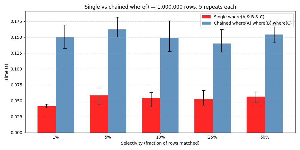
Combining filters is 4x faster than chaining them
It is tempting to filter a CTable step by step — first narrow by one condition, then filter the result by another. But each where() call creates a new view with its own mask computation. A single where() with all conditions joined by & does the same work in one pass and is 4.4x faster than five chained calls returning the same final result.
Memory footprint depends on your data
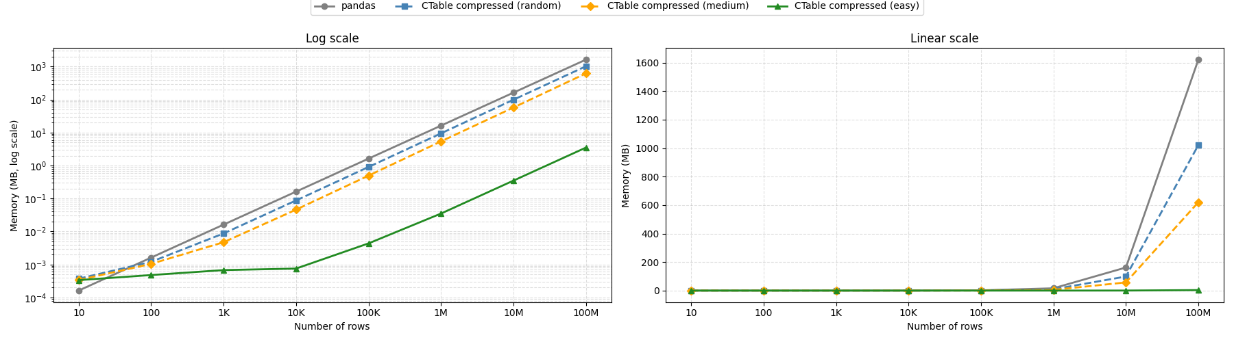
CTable compresses each column independently with Blosc2, so how much memory you save depends on how much structure your data has. With highly repetitive data — sequential integer IDs, a handful of distinct float values, constant booleans — a 100-million-row table fits in under 4 MB, versus over 1.6 GB for the equivalent pandas DataFrame. With fully random data the gain is more modest (around 1.6×), since high-entropy values leave little for the compressor to exploit. Real-world datasets typically land somewhere in between, but CTable is consistently more memory-efficient than pandas regardless of data entropy.
Efficient Indexing
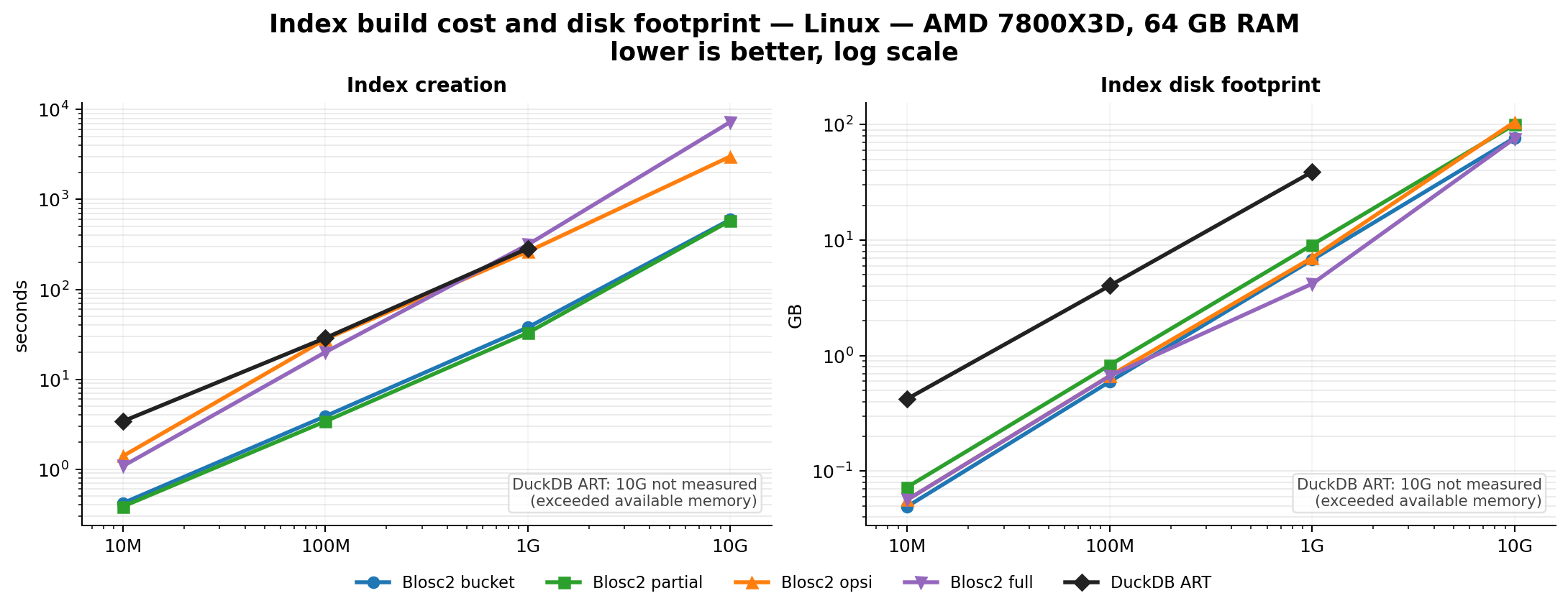
Indexes can speed up queries by orders of magnitude. The embedded indexing engine stores data in compressed form, allowing for large savings in memory and disk. For example, a FULL index on a 1 billion rows with random values takes around 5.8 GB on disk, while an equivalent DuckDB index takes around 41 GB. Typically, queries that would take seconds can be reduced to milliseconds.
Schema validation has near-zero cost at scale
Every CTable has a typed schema with optional constraints (ranges, string lengths, etc.). When inserting data with extend(), these constraints are checked via a vectorized NumPy path rather than row by row. At 1M rows with a NumPy structured array the validation overhead is essentially 1.00x —indistinguishable from skipping validation entirely. Even with Python list input it only adds 1.31x. You get correctness guarantees without paying for them at scale.
AI role
During the development of CTable, we have been using AI tools to help us in the design and implementation of the API, as well as in the documentation. Tools like Perplexity, and agents like Pi, Codex or Claude have been instrumental in helping us throughout the process, which allowed us to be much more ambitious in the features we wanted to implement. Note from Francesc: I specially liked the combination of the Pi agent and GPT 5.5 model (essentially GPT >= 5.3); that worked really well!
Of course, we already borrowed some ideas from other libraries, like Apache Arrow, Pandas, Polars, DuckDB or PyTables, but we also wanted to bring some unique features to CTable, like the ability to operate on compressed data without decompressing it, or the rich schema specs for expressing complex data types; AI has been instrumental in allowing us doing this.
Being a powerful tool, AI always need supervision and guidance to be used effectively, and we have spent lots of time bringing our cumulated decades-long experience for review code, designing tests and benchmarks, and fine-tuning the internal knobs for allowing best performance and user experience. We must say that we are very happy with the results: combining our experience with the power of AI has allowed us to create a powerful and flexible tabular data container that is well tested and documented.
More info
We have setup a couple of tutorials and a complete API reference to get you started with CTable:
CTable brings together compression, schema validation, and query acceleration in a self-contained Python package. It is still young, but the architecture is solid and the feature set already covers most common analytical workflows, and we hope it will be useful for many users in the Python ecosystem. We are looking forward to seeing how the community will use and contribute to Python-Blosc2 in general, an CTable in particular, and to continue improving it based on feedback and contributions from users.
As mentioned in previous blog posts (see this blog) the maintainers of python-blosc2 are going all-in on Array API integration. This means adding new functions to bring the library up to the standard. Of course, integrating a given function may be more or less difficult for a given library which aspires to compatibility, depending on legacy code, design principles, and the overarching philosophy of the package. Since python-blosc2 uses chunked arrays, handling reductions and mapping between local chunk- and global array-indexing can be tricky. We had some help from Yang Kang Chua at UConn with this functionality - many thanks to him!
Cumulative reductions
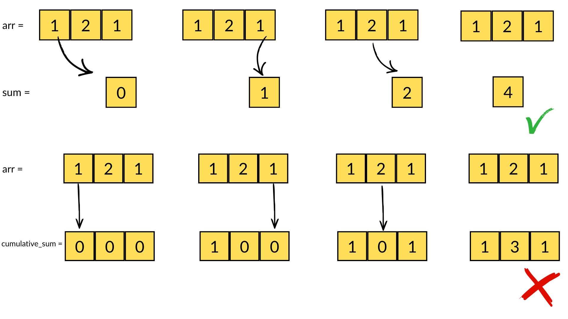
Consider an array a of shape (1000, 2000, 3000) and data type float64 (more on numerical precision later). The result of sum(a, axis=0) would be (20, 30) and sum(a, axis=1) would be (1000, 3000). In general we can say that reductions reduce the sizes of arrays. On the other hand, cumulative reductions store the intermediate reduction results along the reduction axis, so that the shape of the result is always the same as that of the input array: cumulative_sum(a, axis=ax) is always (1000, 2000, 3000) for any (valid) value of ax.
This has a couple of consequences. One is that memory consumption may be rather important: the array a will occupy math.prod((1000, 2000, 3000))*8/(1024**3) = 44.7GB, but its sum along the first axis only .0447GB. Thus we can easily store the final result in memory. Not so for the result of cumulative_sum which also occupies 44.7GB!
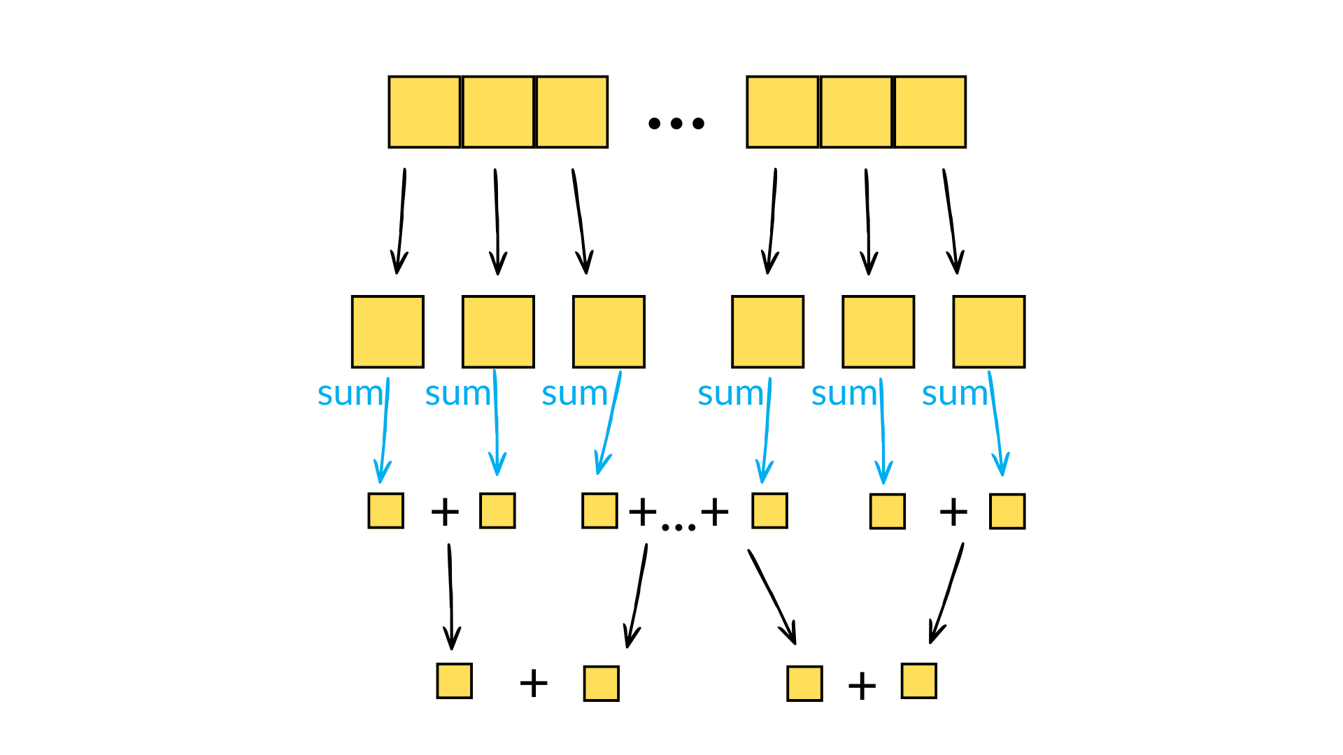
The second consequence, for chunked array libraries, is that the order in which one loads chunks and calculates the result matters. Consider the following diagram, where we have a 1D array of three elements. To calculate the final sum, we may load the chunks in any order and do not require access to any previous value except the running total - loading the first, third and finally second chunks, we obtain the correct sum of 4. However, for the cumulative sum, each element of the result depends on the previous element (and from there the sum of all prior elements of the array). Consequently, we must ensure we load the chunks according to their order in memory - if not, we will end up with an incorrect final result. A minimal criterion is that the final element of the cumulative sum should be the same as the sum, which is not the case here!
Consequences for numerical precision
When calculating reductions, numerical precision is a common hiccup. For products, one can quickly overflow the data type - the product of arange(1, 14) already overflows the maximum value of int32. For sums, rounding errors incurred due to adding elements of a small size to the running total of a large size can quickly become significant. For this reason, Numpy will try to use pairwise summation to calculate sum(a) - this involves breaking the array into small parts, calculating the sum on each small part (i.e. simply successively adding elements to a running total), and then recursively summing pairs of sums until the final result is reached. Each recursive sum operation thus involves the sum of two numbers of similar size, thus reducing the rounding errors incurred when summing disparate numbers. This algorithm also only has a minimal additional overhead compared to the naive approach and is eminently parallelisable. And it has a natural recursive implementation, something which computer scientists always find appealing even if only for aesthetic reasons!
Unfortunately, such an approach is not possible for cumulative sums since, as discussed above, order matters! One possibility is to use Kahan summation (the Wikipedia article is excellent), which does have additional costs (both in terms of FLOPS and memory consumption) although these are not prohibitive. One essentially keeps track of the rounding errors incurred with an auxiliary running total and uses this to correct the sum:
# Kahan summation algorithmtot=0tracker=0forelinarray:corrected_el=el-c# nudge el with accumulated lost digitstemp=tot+corrected_el# lose last few digits of eltracker=(temp-tot)-corrected_el# store the lost digits of eltot=temp
In implementation, we calculate the cumulative sum on a decompressed chunk in order and then carry forward the last element of the cumulative sum (i.e. the sum of the whole chunk) to the next chunk, incrementing the result of the cumulative sum by this carried-over value to give the global cumulative sum. Thus, we can use Kahan summation between the small(er) values of the local chunk cumulative sum and the large(r) carried-forward running total to try and conserve precision.
Unfortunately, we still observe discrepancies with respect to the Numpy implementation (which sums element-by-element essentially) of cumulative sum - but this also differs from the results of np.sum due to the latter's use of pairwise summation! Finite arithmetic imposes an insuperable barrier: three different algorithms cannot guarantee agreement in every possible case. Since the Kahan sum approach has a slight overhead, we decided to junk it, as it did not improve precision sufficiently to justify its use.
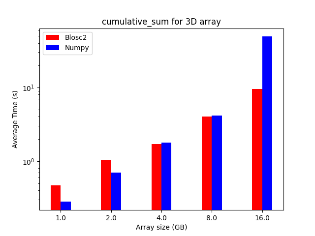
Experiments
We performed some experiments comparing the new blosc2.cumulative_sum function to Numpy's version for some large arrays of (of size (N, N, N) for various values of N). Since the working set is double the size of the input array (input + output), we expect to see significant benefits from Blosc2 compression and exploitation of caching. Indeed, once the working set size starts to approach the available RAM (32 GB), NumPy begins to slow down rapidly and when the working set exceeds memory and swap must be used NumPy becomes vastly slower.
The plot shows the average computation time for cumulative_sum over the three different axes of the input array. The benchmark code may be found here.
Conclusions
Blosc2 achieves superior compression and enables computation on larger datasets by tightly integrating compression and computation and interleaving I/O and computation. The returns on such an approach are clear in an era of increasingly expensive RAM and thus increasingly desirable memory efficiency. As an array library catering in a unique way to this growing need, bringing Blosc2 into greater alignment with the interlibrary array API standard is of utmost importance to ease its integration into users' workflows and applications. We are thus especially pleased that the performance of the freshly-implemented cumulative reduction operations mandated by the Array API standard only underline the validity of chunkwise operations.
The Blosc team isn't resting on our laurels either, as we continue to optimise the existing framework to accelerate computations further. The recent introduction of the miniexpr library into the backend is the capstone to these efforts, and has made the compression/computation integration truly seamless, bringing incredible speedups for memory-bound computations, justifying Blosc2's compression-first, cache-aware philosophy. This all allows Blosc2 to handle significantly larger working sets than other solutions, delivering high performance for both in-memory and on-disk datasets, even exceeding available RAM.
If you find our work useful and valuable, we would be grateful if you could support us by making a donation. Your contribution will help us continue to develop and improve Blosc packages, making them more accessible and useful for everyone. Our team is committed to creating high-quality and efficient software, and your support will help us to achieve this goal.
Blosc's philosophy of meta-compression is incredibly powerful - one is able to compose pipelines to optimally compress data (for speed or compression ratio), store information about the pipeline alognside the data in metadata, and then rely on a generic decompressor to read this and reverse the pipeline. The OpenZL team share our belief in the validity of this approach and have designed a graph-based formalisation with extensive support for all kinds of compression pipelines for all kinds of data.
However, Blosc2 is now much more than just a compression library - it offers comprehensive indexing support (including fancy indexing via the python-blosc2 interface) as well as an increasingly rapid compute engine (see this blog!). What if we could marry the incredibly comprehensive compression coverage of OpenZL with Blosc2's extended array manipulation functionality?
Foreseeing precisely this sort of challenge, prior Blosc2 developers implemented a dynamic plugin register functionality (loading the plugin in C-Blosc2, which can be called via Python-Blosc2). This means that with some unintrusive, relatively concise interface code, one can link Blosc2 and OpenZL at runtime (without substantially modifying either) and offer Blosc2 arrays compressed and decompressed with OpenZL.
The OpenZL plugin
The source code for the plugin can be found here. The minimal skeleton for the plugin layout follows
The header blosc2_openzl.h then makes the info and encoder/decoder functions available to Blosc2:
#include "blosc2.h"
#include "blosc2/codecs-registry.h"
#include "openzl/openzl.h"

BLOSC2_OPENZL_EXPORT int blosc2_openzl_encoder(...);

BLOSC2_OPENZL_EXPORT int blosc2_openzl_decoder(...);

// Declare the info struct as extern
extern BLOSC2_OPENZL_EXPORT codec_info info;
PEP 427 and wheel structure
In order for the plugin to dynamically link to Blosc2, it has to be able to find the Blosc2 library at runtime. This has historically been quite finicky since different platforms and package managers may store Python packages (and the associated .so/.dylib/.dll library objects differently). Consequently, PEP 427 recommends distributing the Python wheels for packages which depend on compiled objects such as Python-Blosc2 in the following way
Note that it is not necessary to link blosc2_openzl and blosc2 in target_link_libraries as the former depends only on macros and structs defined in header files - and not functions. This makes the libblosc2_openzl.so object especially light and robust, as blosc2 is not registered as an explicit dependency. In fact on Linux, even if the blosc2_openzl.c were to include blosc2 functions, it is still not necessary to perform such linking!
Following PEP 427 allows one to add an additional safeguard to check if the plugin fails to find blosc2 by adding the RUNTIME_PATH property to the installed object
It also allows one to easily find the plugin .so object when calling via python - in the blosc2_openzl/__init__.py file one can find the library path as easily as os.path.abspath(Path(__file__).parent / libname) where libname is the desired .so/.dylib/.dll object (depending on platform). All these benefits have led us to update the wheel structure for python-blosc2 in the latest 4.0 release.
Using OpenZL from Python
Installing is then as simple as:
pip install blosc2_openzl
One can also download the project and use the cmake and cmake --build commands to compile C-level tests or examples. But let's get compressing with python straight away:
import blosc2
import numpy as np
import blosc2_openzl
from blosc2_openzl import OpenZLProfile as OZLP
prof = OZLP.OZLPROF_SH_BD_LZ4
# Define the compression parameters for Blosc2
cparams = {'codec': blosc2.Codec.OPENZL, 'codec_meta': prof.value}

# Create (uncompressed) array
np_array = np.arange(1000).reshape((10,100))

# Compression with the OpenZL codec
bl_array = blosc2.asarray(np_array, cparams=cparams)
print(bl_array.cratio) # print compression ratio
>> 25.078369905956112
The OpenZLProfile enum contains the available profile pipelines that have been implemented in the plugin, which use the codec_meta field (an 8-bit integer) to specify the desired transformation via codecs, filters and other nodes for the compression graph. Starting from the Least-Significant-Bit (LSB), setting the bits tells OpenZL how to build the graph:
CODEC | SHUFFLE | DELTA | SPLIT | CRC | x | x | x |
CODEC - If set, use LZ4. Else ZSTD.
SHUFFLE - If set, use shuffle (outputs a stream for every byte of input data typesize)
DELTA - If set, apply a bytedelta (to all streams if necessary)
SPLIT - If set, do not recombine the byte streams
CRC - If set, store a checksum during compression and check it during decompression
The remaining bits may be used in the future.
In the future it would be great to further expand the OpenZL functionalities that we can offer via the plugin, such as bespoke transformers trained via machine learning techniques - see the OpenZL page for a flavour of what can be done with the (still evolving) library.
Conclusions
C-Blosc2's ability to support dynamically loaded plugins allows the library to grow in features without increasing the size and complexity of the library itself. For more information about user-defined plugins, refer to this blog entry. We have put this to work to offer linkage with the rather complex OpenZL library with a relatively rapid turnaround from design to prototype to full release in around a month. This is thanks to prior hard work by open source contributors from Blosc but naturally also OpenZL - many thanks to all!
If you find our work useful and valuable, we would be grateful if you could support us by making a donation. Your contribution will help us continue to develop and improve Blosc packages, making them more accessible and useful for everyone. Our team is committed to creating high-quality and efficient software, and your support will help us to achieve this goal.
Can a library designed for computing with compressed data ever hope to outperform highly optimized numerical engines like NumPy and Numexpr? The answer is complex, and it hinges on the "memory wall" — a phenomenon which occurs when system memory limitations start to drag on CPU. This post uses Roofline analysis to explore this very question, dissecting the performance of Blosc2 and revealing the surprising scenarios where it can gain a competitive edge.
TL;DR
Before we dive in, here's what we discovered:
For in-memory tasks, Blosc2's overhead can make it slower than Numexpr, especially on x86 CPUs.
This changes on Apple Silicon, where Blosc2's performance is much more competitive.
For on-disk tasks, Blosc2 consistently outperforms NumPy/Numexpr on both platforms.
The "memory wall" is real, and disk I/O is an even bigger one, which is where compression shines.
A Trip Down Memory Lane
Let's rewind to 2008. NumPy 1.0 was just a toddler, and the computing world was buzzing with the arrival of multi-core CPUs and their shiny new SIMD instructions. On the NumPy mailing list, a group of us were brainstorming how to harness this new power to make Python's number-crunching faster.
The idea seemed simple: trust newer compilers to use SIMD (and, possibly, data alignment) to perform operations on multiple data points at once. To test this, a simple benchmark was shared: multiply two large vectors element-wise. Developers from around the community ran the code and shared their results. What came back was a revelation.
For small arrays that fit snugly into the CPU's high-speed cache, SIMD was quite good at accelerating computations. But as soon as the arrays grew larger, the performance boost vanished. Some of us were already suspicious about the new "memory wall" that had been growing lately, seemingly due to the widening gap between CPU speeds and memory bandwidth. However, a conclusive answer (and solution) was still lacking.
But amidst the confusion, a curious anomaly emerged. One machine, belonging to NumPy legend Charles Harris, was consistently outperforming the rest—even those with faster processors. It made no sense. We checked our code, our compilers, everything. Yet, his machine remained inexplicably faster. The answer, when it finally came, wasn't in the software at all. Charles, a hardware wizard, had tinkered with his BIOS to overclock his RAM from 667 MHz to a whopping 800 MHz.
That was my lightbulb moment: for data-intensive tasks, raw CPU clock speed was not the limiting factor; memory bandwidth was what truly mattered.
This led me to a wild idea: what if we could make memory effectively faster? What if we could compress data in memory and decompress it on-the-fly, just in time for the CPU? This would slash the amount of data being moved, boosting our effective memory bandwidth. That idea became the seed for Blosc, a project I started in 2010 that has been my passion ever since. Now, 15 years later, it is time to revisit that idea and see how well it holds up in today's computing landscape.
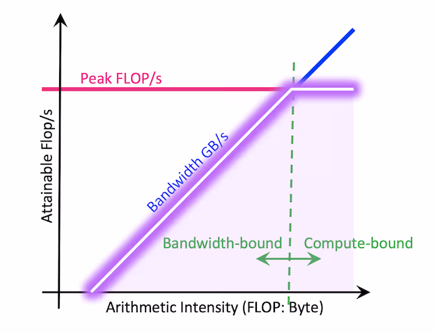
Roofline Model: Understanding the Memory Wall
Not all computations are equally affected by the memory wall - in general performance can be either CPU-bound or memory-bound. To diagnose which resource is the limiting factor, the Roofline model provides an insightful analytical framework. This model plots computational performance against arithmetic intensity (i.e. floating-point operations per second versus memory accesses per second) to visually determine whether a task is constrained by CPU speed or memory bandwidth.
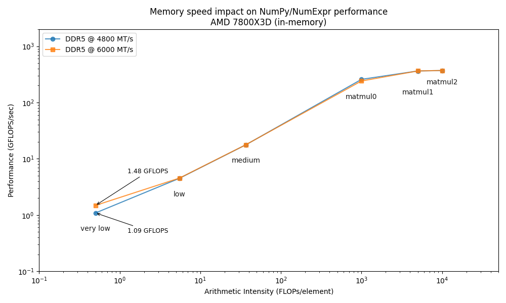
We will use Roofline plots to analyze Blosc2's performance, compared to that of NumPy and Numexpr. NumPy, with its highly optimized linear algebra backends, and Numexpr, with its efficient evaluation of element-wise expressions, together form a strong performance baseline for the full range of arithmetic intensities tested.
To highlight the role of memory bandwidth, we will conduct our benchmarks on an AMD Ryzen 7800X3D CPU at two different memory speeds: the standard 4800 MTS and an overclocked 6000 MTS. This allows us to directly observe how memory frequency impacts computational performance.
To cover a range of computational scenarios, our benchmarks include five operations with varying arithmetic intensities:
Very Low: A simple element-wise addition (a + b + c).
Low: A moderately complex element-wise expression (sqrt(a + 2 * b + (c / 2)) ^ 1.2).
Medium: A highly complex element-wise calculation involving trigonometric and exponential functions.
High: Matrix multiplication on small matrices (labeled matmul0).
Very High: Matrix multiplication on large matrices (labeled matmul1 and matmul2).
The Roofline plot confirms that increasing memory speed only benefits memory-bound operations (low arithmetic intensity), while CPU-bound tasks (high arithmetic intensity) are unaffected, as expected. Although this might suggest the "memory wall" is not a major obstacle, low-intensity operations like element-wise calculations, reductions, and selections are extremely common and often create performance bottlenecks. Therefore, optimizing for memory performance remains crucial.
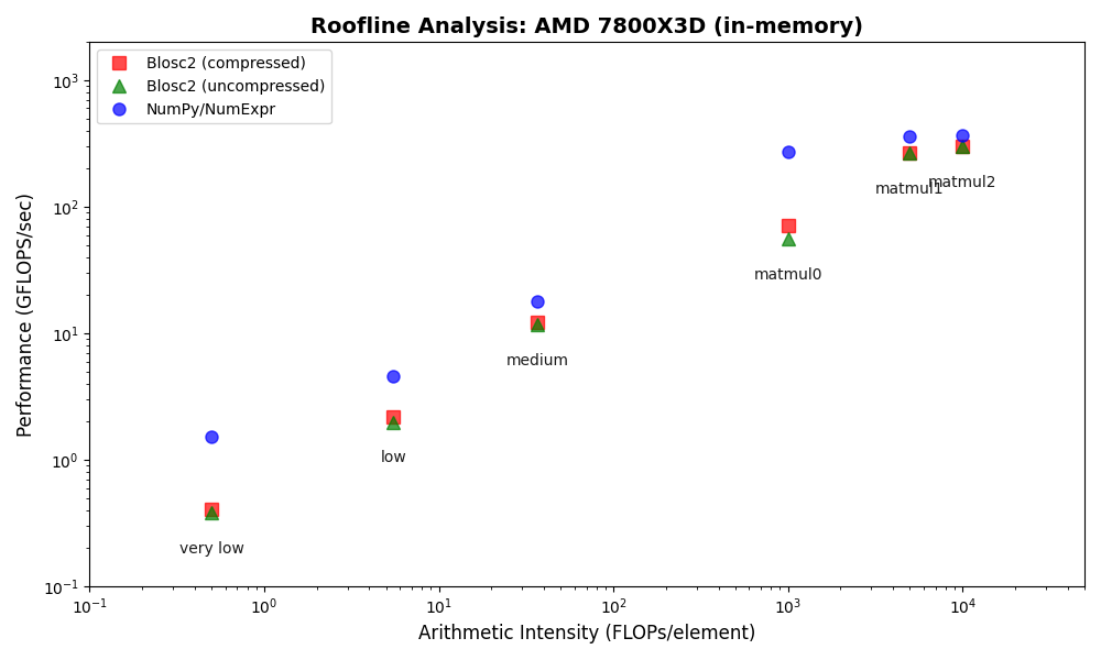
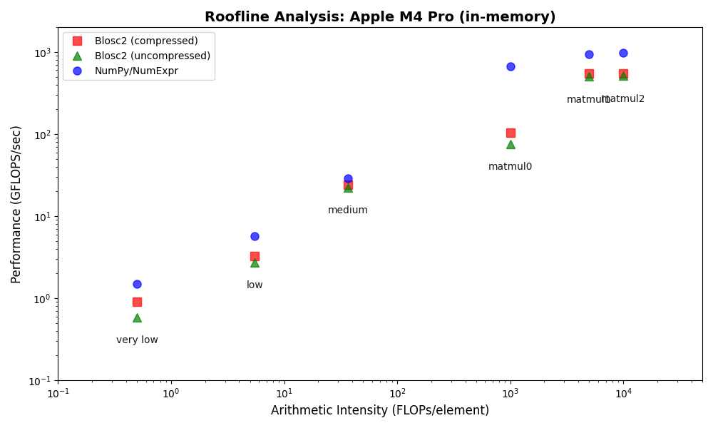
The In-Memory Surprise: Why Wasn't Compression Faster?
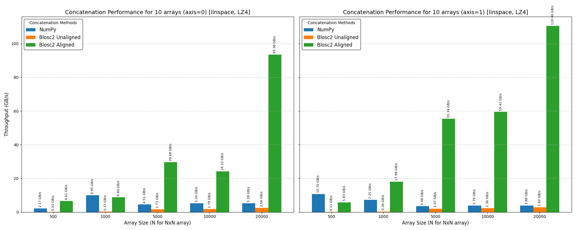
We benchmarked Blosc2 (both compressed and uncompressed) against NumPy and Numexpr. For this test, Blosc2 was configured with the LZ4 codec and shuffle filter, a setup known for its balance of speed and compression ratio. The benchmarks were executed on an AMD Ryzen 7800X3D CPU with memory speed set to 6000 MTS, ensuring optimal memory bandwidth for the tests.
The analysis reveals a surprising outcome: for memory-bound operations, Blosc2 is up to five times slower than Numexpr. Although operating on compressed data provides a marginal improvement over uncompressed Blosc2, it is not enough to overcome this performance gap. This result is unexpected because Blosc2 leverages Numexpr internally, and the reduced memory bandwidth from compression should theoretically lead to better performance in these scenarios.
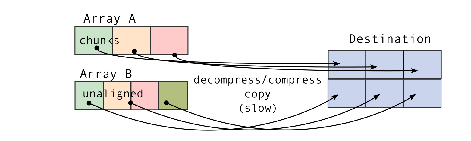
To understand this counter-intuitive result, we must examine Blosc2's core architecture. The key lies in its double partitioning scheme, which, while powerful, introduces an overhead that can negate the benefits of compression in memory-bound contexts.
Unpacking the Overhead: A Look Inside Blosc2's Architecture
The performance characteristics of Blosc2 are rooted in its double partitioning architecture, which organizes data into chunks and blocks.
This design is crucial for both aligning with the CPU's memory hierarchy and enabling efficient multidimensional array representation (important for things like e.g. n-dimensional slicing). However, this structure introduces an inherent overhead from additional indexing logic. In memory-bound scenarios, this latency counteracts the performance gains from reduced memory traffic, explaining why Blosc2 does not surpass Numexpr.
Conversely, as arithmetic intensity increases, the computational demands begin to dominate the total execution time. In these CPU-bound regimes, the partitioning overhead is effectively amortized, allowing Blosc2 to close the performance gap and eventually match NumPy's performance in tasks like large matrix multiplications.
Modern ARM Architectures
CPU architecture is a rapidly evolving field. To investigate how these changes impact performance, we extended our analysis to the Apple Silicon M4 Pro, a modern ARM-based processor.
The results show that Blosc2 performs significantly better on this platform, narrowing the performance gap with NumPy/NumExpr, especially for operations on compressed data. While compute engines optimized for uncompressed data still hold an edge, these findings suggest that compression will play an increasingly important role in improving computational performance in the future.
However, while the in-memory results are revealing, they don't tell the whole story. Blosc2 was designed not just to fight the memory wall, but to conquer an even greater bottleneck: disk I/O. Although compression has the benefit of fitting more data into RAM when used in-memory (which is per se extremely interesting in these times, where RAM prices skyrocketed), its true power is unleashed when computations move off-motherboard. Now, let's shift the battlefield to the disk and see how Blosc2 performs in its native territory.
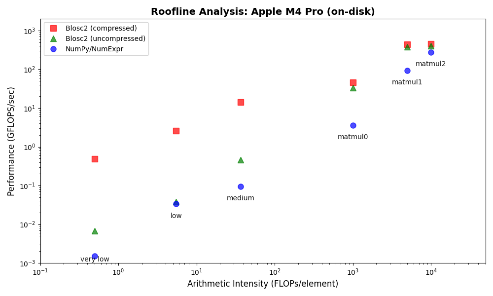
A Different Battlefield: Blosc2 Shines with On-Disk Data
Blosc2's architecture extends its computational engine to operate seamlessly on data stored on disk, a significant advantage for large-scale analysis. This is particularly relevant in scenarios where datasets exceed available memory, necessitating out-of-core processing, as commonly encountered in data science, machine learning workflows or cloud computing environments.
Our on-disk benchmarks were designed to use datasets larger than the system's available memory to prevent filesystem caching from influencing the results. To establish a baseline, we implemented an out-of-core solution for NumPy/NumExpr, leveraging memory-mapped files. Here Blosc2 has a performance edge, particularly for memory-bound operations on compressed data, being able to send and receive data faster to disk than the memory-mapped NumPy arrays.
In this case, we've used high-performance NVMe SSDs (NVMe 4.0) to minimize the impact of disk speed on the results. We also switched to the ZSTD codec for Blosc2, as its superior compression ratio over LZ4 further minimizes data transfer to and from the disk.
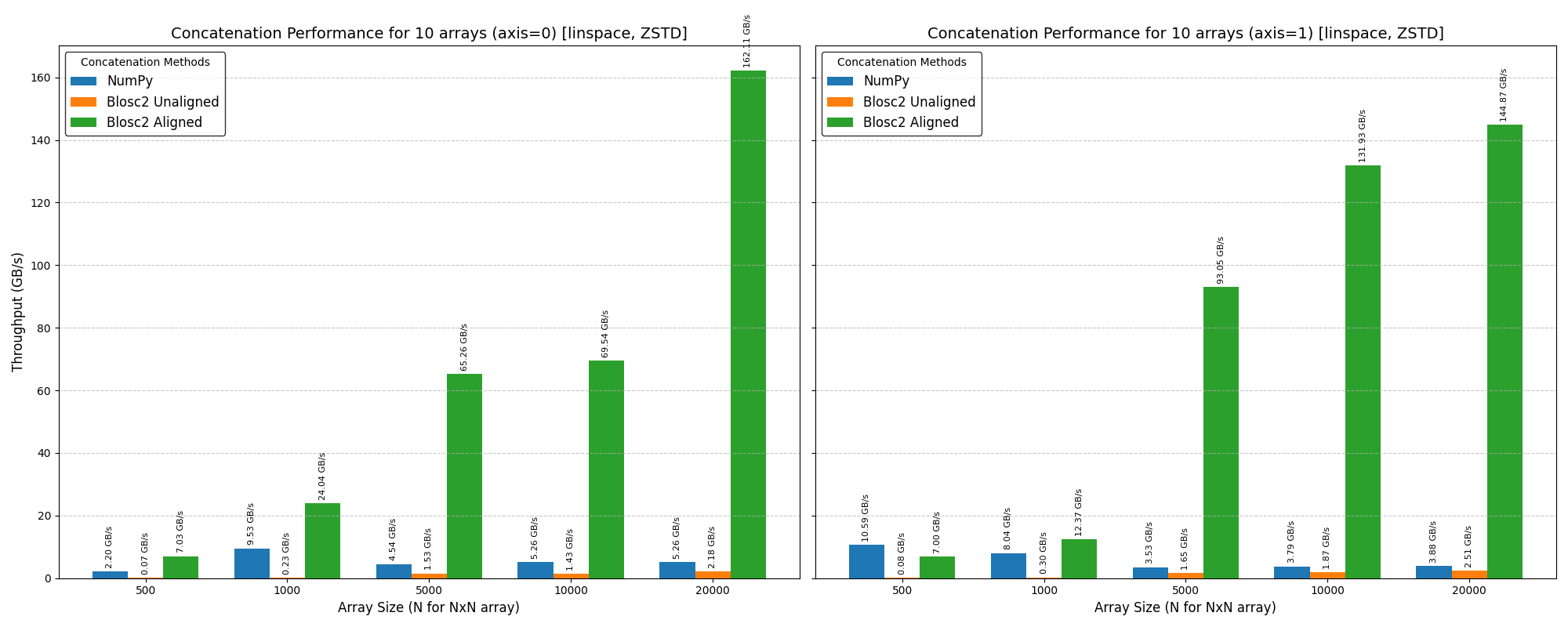
First, let's see the results for the AMD Ryzen 7800X3D system:
The plots above show that Blosc2 outperforms both NumPy and Numexpr for all low-to-medium intensity operations. This is because the high latency of disk I/O amortizes the overhead of Blosc2's double partitioning scheme. Furthermore, the reduced bandwidth required for compressed data gives Blosc2 an additional performance advantage in this scenario.
Now, let's see the results for the Apple Silicon M4 Pro system:
On the Apple Silicon M4 Pro system, Blosc2 again outperforms both NumPy and Numexpr for all on-disk operations, mirroring the results from the AMD system. However, the performance advantage is even more significant here, especially for memory-bound tasks. This is mainly because memory-mapped arrays are less efficient on Apple Silicon than on x86_64 systems, increasing the overhead for the NumPy/Numexpr baseline.
Roofline Plot: In-Memory vs On-Disk
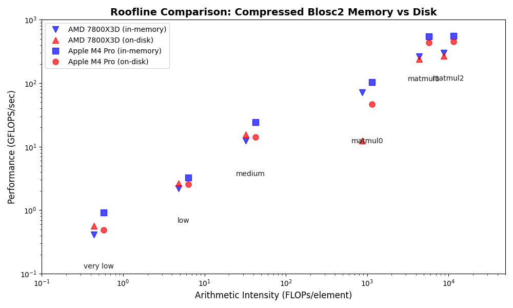
To better understand the trade-offs between in-memory and on-disk processing with Blosc2, the following plot contrasts their performance characteristics for compressed data:
A notable finding for the AMD system is that Blosc2's on-disk operations are noticeably faster than its in-memory operations, especially for memory-bound tasks (low arithmetic intensity). This is likely due to two factors: first, the larger datasets used for on-disk tests allow Blosc2 to use more efficient internal partitions (chunks and blocks), and second, parallel data reads from disk further reduce bandwidth requirements.
In contrast, for CPU-bound tasks (high arithmetic intensity), on-disk performance is comparable to, albeit slightly slower than, in-memory performance. The analysis also reveals a specific weakness: small matrix multiplications (matmul0) are significantly slower on-disk, identifying a clear target for future optimization.
In contrast to the AMD system, the Apple Silicon M4 Pro shows that Blosc2's on-disk operations are slower than in-memory, a difference that is most significant for memory-bound tasks. This performance disparity suggests that current on-disk optimizations may favor x86_64 architectures over ARM.
As with the AMD platform, CPU-bound operations exhibit similar performance for both on-disk and in-memory contexts. The notable exception remains the small matrix multiplication (matmul0), which performs significantly worse on-disk. This recurring pattern pinpoints a clear opportunity for future optimization efforts.
Finally, and in addition to its on-disk performance, Blosc2 offers a significant cost advantage. With the recent rise in SSD prices, compressing data on disk becomes an economically attractive strategy, allowing you to store more data in less space and thereby reduce hardware expenses.
Reproducibility
All the benchmarks and plots presented in this blog post can be reproduced. You are invited to run the scripts on your own hardware to explore the performance characteristics of Blosc2 in different environments. In case you get interesting results, please consider sharing them with the community!
Conclusions
In this blog post, we explored the Roofline model to analyze the performance of Blosc2, NumPy, and Numexpr. We've confirmed that memory-bound operations are significantly affected by the "memory wall", making data compression of interest when maximizing performance. However, for in-memory operations, the overhead of Blosc2's double partitioning scheme can be a limiting factor, especially on x86_64 architectures. Encouragingly, this performance gap narrows considerably on modern ARM platforms like Apple Silicon, suggesting a promising future.
The situation changes dramatically for on-disk operations. Here, Blosc2 consistently outperforms NumPy and Numexpr, as the high latency of disk I/O (even if we used SSDs here) amortizes its internal overhead. This makes Blosc2 a compelling choice for out-of-core computations, one of its primary use cases.
Overall, this analysis has provided valuable insights, highlighting the importance of the memory hierarchy. It has also exposed specific areas for improvement, such as the performance of small matrix multiplications. As Blosc2 continues to evolve, I am confident we can address these points and further enhance its performance, making it an even more powerful tool for numerical computations in Python.
Read more about ironArray SLU — the company behind Blosc2, Caterva2, Numexpr and other high-performance data processing libraries.
While compression is often seen merely as a way to save storage, the Blosc development team has long viewed it as a foundational element for high-performance computing. This philosophy is at the heart of Blosc2, which is not just a compression library but a powerful framework for handling large datasets. This post will highlight one of Python-Blosc2's most exciting capabilities: its lazy evaluation engine for array operations.
Libraries optimised for computation on large datasets that don't fit in memory - such as Dask or Spark - often use lazy evaluation of computation expressions. This typically speeds up evaluation since one can build the full chain of computations and only execute them when the final result is needed. Consequently, Python-Blosc2's compute engine also uses the lazy imperative paradigm, which proves to be both powerful and efficient.
An additional benefit of the engine is its ability to act as a universal backend. Python-Blosc2 has a native blosc2.NDArray format, but it can also easily execute lazy operations on arrays from other popular libraries like NumPy, HDF5, Zarr, Xarray or TileDB - basically any array object which complies with a minimal protocol.
In the recent Python-Blosc2 3.10.x series, we added support for lazy evaluation of eager functions, expanding the capabilities of the compute engine, and making interaction with other formats easier. Let's explore how this works using an out-of-core tensordot operation as an example.
From Eager to Lazy with blosc2.lazyexpr
Functions which return a result with a different shape to the input operands - such as reductions or linear algebra operations - must be evaluated eagerly (computed and the result returned immediately). For example, blosc2.tensordot() executes eagerly.
Nevertheless, we can defer this computation, by wrapping the call in a string and passing it to blosc2.lazyexpr. This creates a LazyExpr object that represents the operation without executing it.
# Assume a and b are large, on-disk blosc2 arraysaxis=(0,1)# Create a lazy expression objectlexpr=blosc2.lazyexpr("tensordot(a, b, axes=(axis, axis))")# The computation has not run yet.# To execute it and save the result to a new persistent array:out_blosc2=lexpr.compute(urlpath="out.b2nd",mode="w")
This is useful, and highly efficient both in terms of computation time and memory usage, as we'll see later. But the real magic happens when we use this computation engine with other array formats.
One Engine, Many Backends
The blosc2.evaluate() function takes the same string expression but can operate on any array-like objects that follow the blosc2.Array protocol. This protocol simply requires the object to have shape, dtype, __getitem__, and __setitem__ attributes, which are standard in h5py, zarr, tiledb, xarray and numpy arrays.
This means you can use Blosc2's efficient evaluation engine to perform out-of-core computations directly on your existing (HDF5, Zarr, etc.) datasets.
Example with HDF5
Here, we instruct blosc2.evaluate to run the tensordot operation on two h5py datasets and store the result in a third one.
# Open HDF5 datasetsf=h5py.File("a_b_out.h5","a")a=f["a"]b=f["b"]out_hdf5=f["out"]# Use blosc2.evaluate() with HDF5 arraysblosc2.evaluate("tensordot(a, b, axes=(axis, axis))",out=out_hdf5)
Notice that the expression string is identical to the one we used before. blosc2 inspects the objects in the expression's namespace and computes with them, regardless of their underlying format.
Example with Zarr
The same principle applies to Zarr arrays.
# Open Zarr arraysa=zarr.open("a.zarr",mode="r")b=zarr.open("b.zarr",mode="r")zout=zarr.open_array("out.zarr",mode="w",...)# Use blosc2.evaluate() with Zarr arraysblosc2.evaluate("tensordot(a, b, axes=(axis, axis))",out=zout)
This makes blosc2.evaluate a powerful, backend-agnostic tool for out-of-core array computations.
Performance Comparison
As well as offering smooth integration, blosc2.evaluate is highly performant. Python-Blosc2 uses a lazy evaluation engine that integrates tightly with the Blosc2 format. This means that the computation is performed on-the-fly, without any intermediate copies. This is a huge advantage for large datasets, as it allows us to perform computations on arrays that don't fit in memory. In addition, it actively tries to leverage the hierarchical memory layout in modern CPUs, so that it can use both private and shared caches in the best way possible.
We ran a benchmark performing a tensordot operation (run over three different axis combinations) on two 3D arrays stored on disk; we then write the output to disk as well.
We consider four approaches:
Blosc2 Native: Using blosc2.lazyexpr with blosc2.NDArray containers.
Blosc2+HDF5: Using blosc2.evaluate with HDF5 for storage.
Blosc2+Zarr: Using blosc2.evaluate with Zarr for storage.
Dask+HDF5: The combination of Dask for computation and HDF5 for storage.
Dask+Zarr: The combination of Dask for computation and Zarr for storage.
For each approach we plot the memory consumption vs. time for arrays of increasing size.
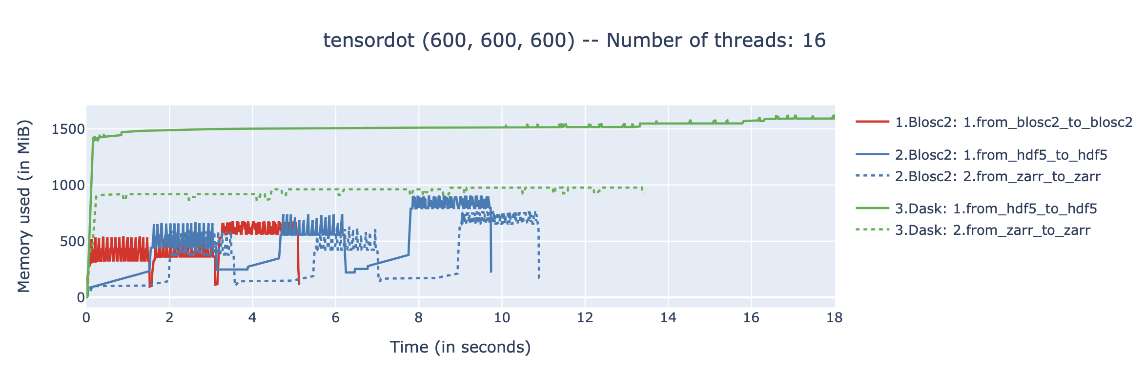
Results on two (600, 600, 600) float64 arrays (3 GB working set):
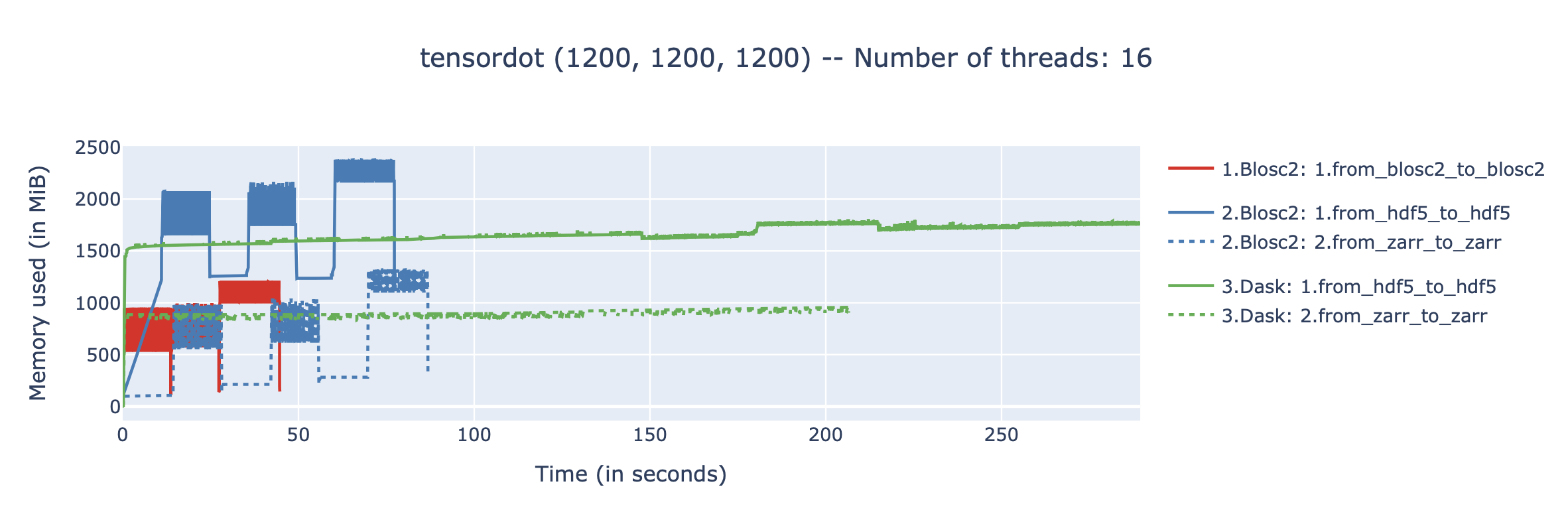
Results on two (1200, 1200, 1200) float64 arrays (26 GB working set):
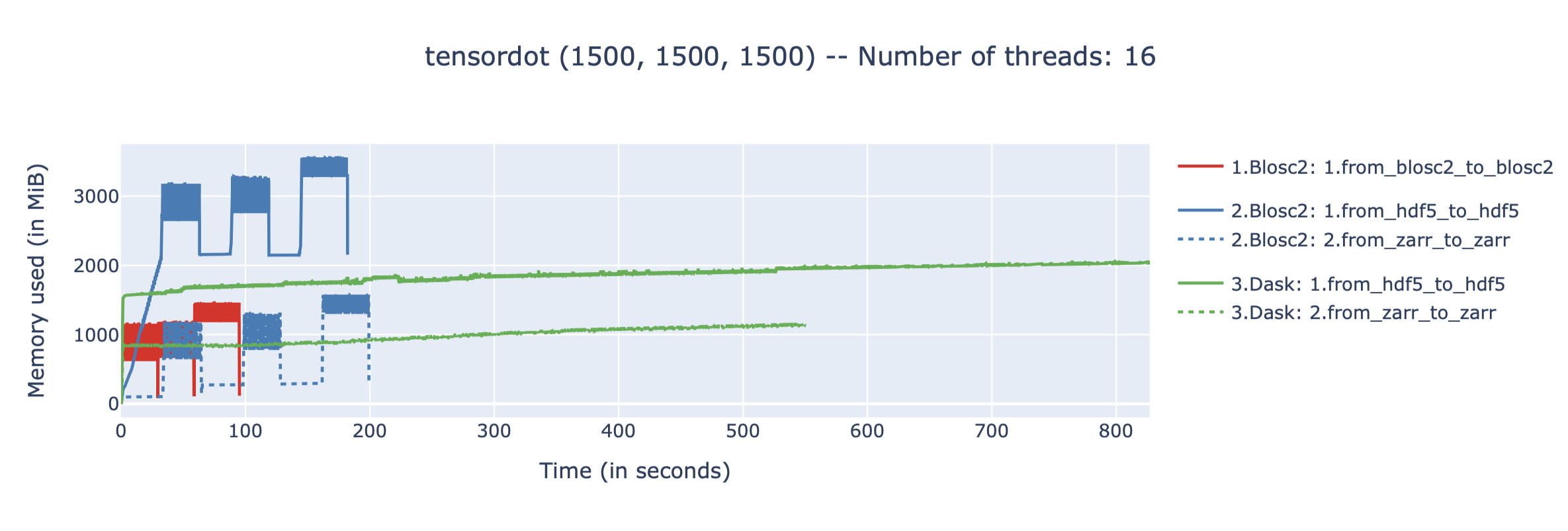
Results on two (1500, 1500, 1500) float64 arrays (50 GB working set):
As can be seen, the amount of memory required by the different approaches is very different, although none requires more than a small fraction of the total working set (which is 3, 26 and 50 GB, respectively). This is because all approaches are out-of-core, and only load small chunks of data into memory at any given time.
The benchmarks were executed on an AMD Ryzen 9800X3D CPU, with 16 logical cores and 64GB of RAM, using Ubuntu Linux 25.04. We have used the following versions of the libraries: python-blosc2 3.10.1, h5py 3.14.0, zarr 3.1.3, 2025.9.1, and numpy 2.3.3. All backends are using Blosc or Blosc2 as the compression backend, with same codecs and filters, and using the same number of threads for compression and decompression.
Analysis
The results are revealing:
Blosc2 native is fastest: The tight integration between the Blosc2 compute engine and its native array format yields the best performance, making it the fastest solution by a significant margin.
Rapid computation time: blosc2.evaluate delivers impressive speed when operating directly on HDF5 and Zarr files, outperforming the more complex Dask+HDF5 and Dask+Zarr stack. This is great news for anyone with existing HDF5/Zarr datasets.
Low memory usage: While the memory consumption for the Blosc2+HDF5 combination is a bit high (we are still analyzing why), the memory usage for the Blosc2 native approach is pretty low, making it suitable for systems with limited RAM and/or operands not fitting in memory.
This is not to say that Dask (or Spark) is an inferior choice for out-of-core computations. It's a great tool for large-scale data processing, especially when using clusters, is very flexible, and offers a wide range of functions; it's certainly a first-class citizen in the PyData ecosystem. However, if your needs are more modest and you want a simple, efficient way to run computations on existing datasets, using a core of common functions, and leveraging the full capabilities of modern multi-core systems, all without the overhead of a full Dask setup, blosc2.evaluate() is a fantastic alternative.
Conclusion
Python-Blosc2 is more than just a compression library for storing data in blosc2.NDArray objects; it's a high-performance computing tool as well. Its lazy evaluation engine provides a simple yet powerful way to handle out-of-core operations. The computation engine is completely decoupled from the compression backend, and thus can easily work with many different array formats; however, the compute engine meshes most tightly with the Blosc2 native array format, achieving maximal performance (in terms of both computation time and memory usage).
By adhering to the Array API standard, it acts as a universal engine that can work with different storage backends; we already implement more than 100 functions that are required by that standard, and the number will only grow in the future. If you have existing datasets in HDF5 or Zarr or TileDB (and we are always looking forward to support even more formats), and need a lightweight, efficient way to run computations on them, blosc2.evaluate() is a fantastic tool to have in your arsenal. Of course, for maximum performance, the native Blosc2 format is a clear winner.
Our work continues. We are committed to enhancing Python-Blosc2 by expanding its supported operations, improving performance across backends, and adding new ones. Stay tuned for more updates! If you found this post useful, please share it. For questions or comments, reach out to us on GitHub.
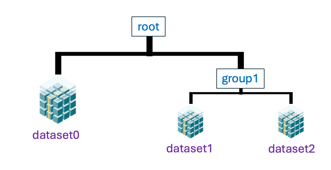
When working with large and complex datasets, having a way to organize your data efficiently is crucial. blosc2.TreeStore is a powerful feature in the blosc2 library that allows you to store and manage your compressed arrays in a hierarchical, tree-like structure, much like a filesystem. This container, typically saved with a .b2z extension, can hold not only blosc2.NDArray or blosc2.SChunk objects but also metadata, making it a versatile tool for data organization.
What is a TreeStore?
A TreeStore lets you arrange your data into groups (like directories) and datasets (like files). Each dataset is a blosc2.NDArray or blosc2.SChunk instance, benefiting from Blosc2's high-performance compression. This structure is ideal for scenarios where data has a natural hierarchy, such as in scientific experiments, simulations, or any project with multiple related datasets.
Basic Usage: Creating and Populating a TreeStore
Creating a TreeStore is straightforward. You can use a with statement to ensure the store is properly managed. Inside the with block, you can create groups and datasets using a path-like syntax.
importblosc2importnumpyasnp# Create a new TreeStorewithblosc2.TreeStore("my_experiment.b2z",mode="w")asts:# You can store numpy arrays, which are converted to blosc2.NDArrayts["/dataset0"]=np.arange(100)# Create a group with a dataset that can be a blosc2 NDArrayts["/group1/dataset1"]=blosc2.zeros((10,))# You can also store blosc2 arrays directly (vlmeta included)ext=blosc2.linspace(0,1,10_000,dtype=np.float32)ext.vlmeta["desc"]="dataset2 metadata"ts["/group1/dataset2"]=ext
In this example, we created a TreeStore in a file named my_experiment.b2z.
It contains two groups, root and group1, each holding datasets.
Reading from a TreeStore
To access the data, you open the TreeStore in read mode ('r') and use the same path-like keys to retrieve your arrays.
# Open the TreeStore in read-only mode ('r')withblosc2.TreeStore("my_experiment.b2z",mode="r")asts:# Access a datasetdataset1=ts["/group1/dataset1"]print("Dataset 1:",dataset1[:])# Use [:] to decompress and get a NumPy array# Access the external array that has been stored internallydataset2=ts["/group1/dataset2"]print("Dataset 2",dataset2[:])print("Dataset 2 metadata:",dataset2.vlmeta[:])# List all paths in the storeprint("Paths in TreeStore:",list(ts))
TreeStore becomes even more powerful when you use metadata and interact with subtrees (groups).
Storing Metadata with vlmeta
You can attach variable-length metadata (vlmeta) to any group or to the root of the tree. This is useful for storing information like author names, dates, or experiment parameters. vlmeta is essentially a dictionary where you can store your metadata.
# Appending metadata to the TreeStorewithblosc2.TreeStore("my_experiment.b2z",mode="a")asts:# 'a' for append/modify# Add metadata to the rootts.vlmeta["author"]="The Blosc Team"ts.vlmeta["date"]="2025-08-17"# Add metadata to a groupts["/group1"].vlmeta["description"]="Data from the first run"# Reading metadatawithblosc2.TreeStore("my_experiment.b2z",mode="r")asts:print("Root metadata:",ts.vlmeta[:])print("Group 1 metadata:",ts["/group1"].vlmeta[:])
Root metadata: {'author': 'The Blosc Team', 'date': '2025-08-17'}
Group 1 metadata: {'description': 'Data from the first run'}
Working with Subtrees (Groups)
A group object can be retrieved from the TreeStore and treated as a smaller, independent TreeStore. This capability is useful for better organizing your data access code.
withblosc2.TreeStore("my_experiment.b2z",mode="r")asts:# Get the group as a subtreegroup1=ts["/group1"]# Now you can access datasets relative to this groupdataset2=group1["dataset2"]print("Dataset 2 from group object:",dataset2[:])# You can also list contents relative to the groupprint("Contents of group1:",list(group1))
Dataset 2 from group object: [0.0000000e+00 1.0001000e-04 2.0002000e-04 ... 9.9979997e-01 9.9989998e-01
 1.0000000e+00]
Contents of group1: ['/dataset2', '/dataset1']
Iterating Through a TreeStore
You can easily iterate through all the nodes in a TreeStore to inspect its contents.
withblosc2.TreeStore("my_experiment.b2z",mode="r")asts:forpath,nodeints.items():ifisinstance(node,blosc2.NDArray):print(f"Found dataset at '{path}' with shape {node.shape}")else:# It's a groupprint(f"Found group at '{path}' with metadata: {node.vlmeta[:]}")
Found dataset at '/group1/dataset2' with shape (10000,)
Found group at '/group1' with metadata: {'description': 'Data from the first run'}
Found dataset at '/group1/dataset1' with shape (10,)
Found dataset at '/dataset0' with shape (100,)
That's it for this introduction to blosc2.TreeStore! You now know how to create, read, and manipulate a hierarchical data structure that can hold compressed datasets and metadata. You can find the source code for this example in the blosc2 repository.
Some Benchmarks
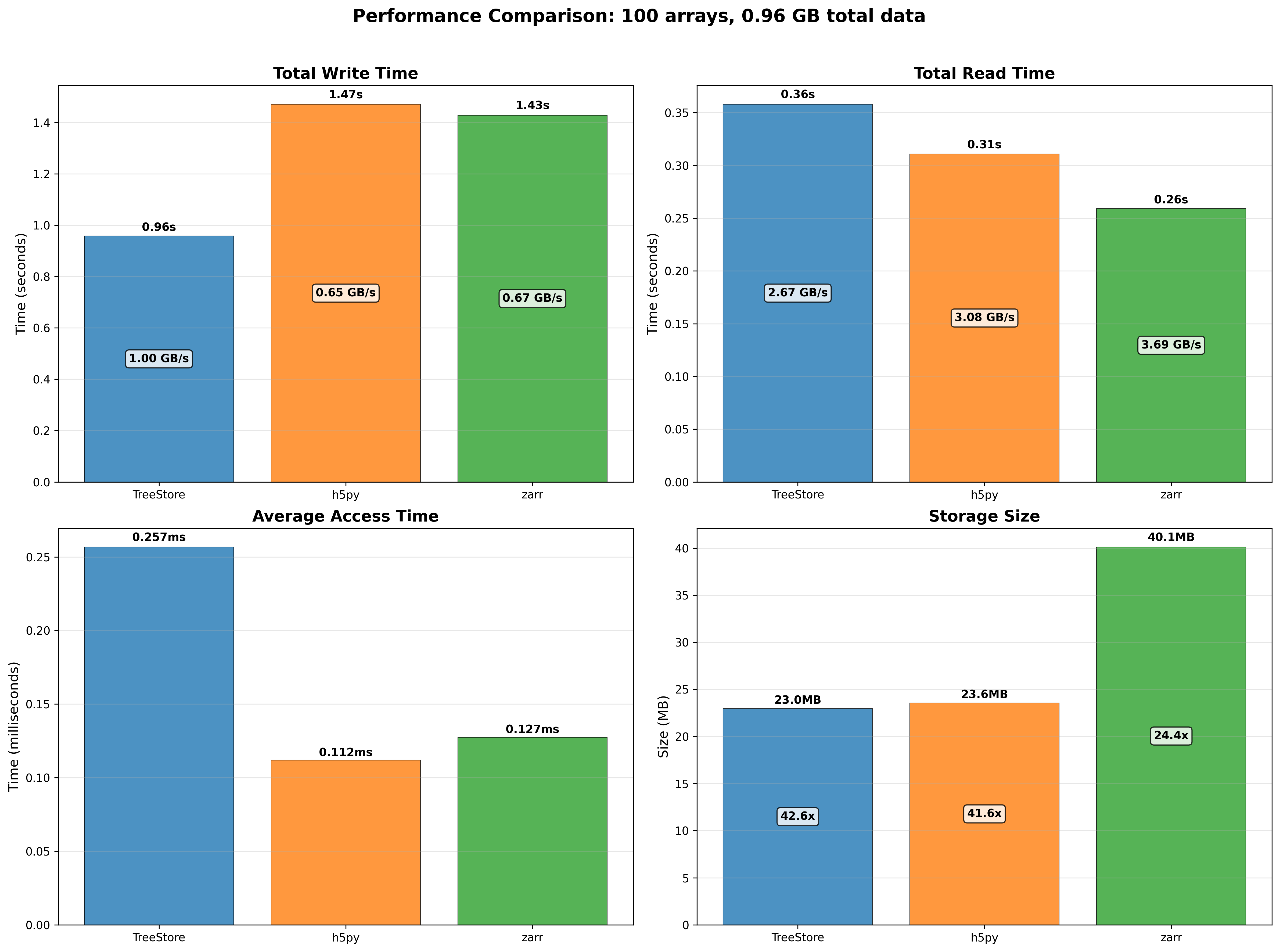
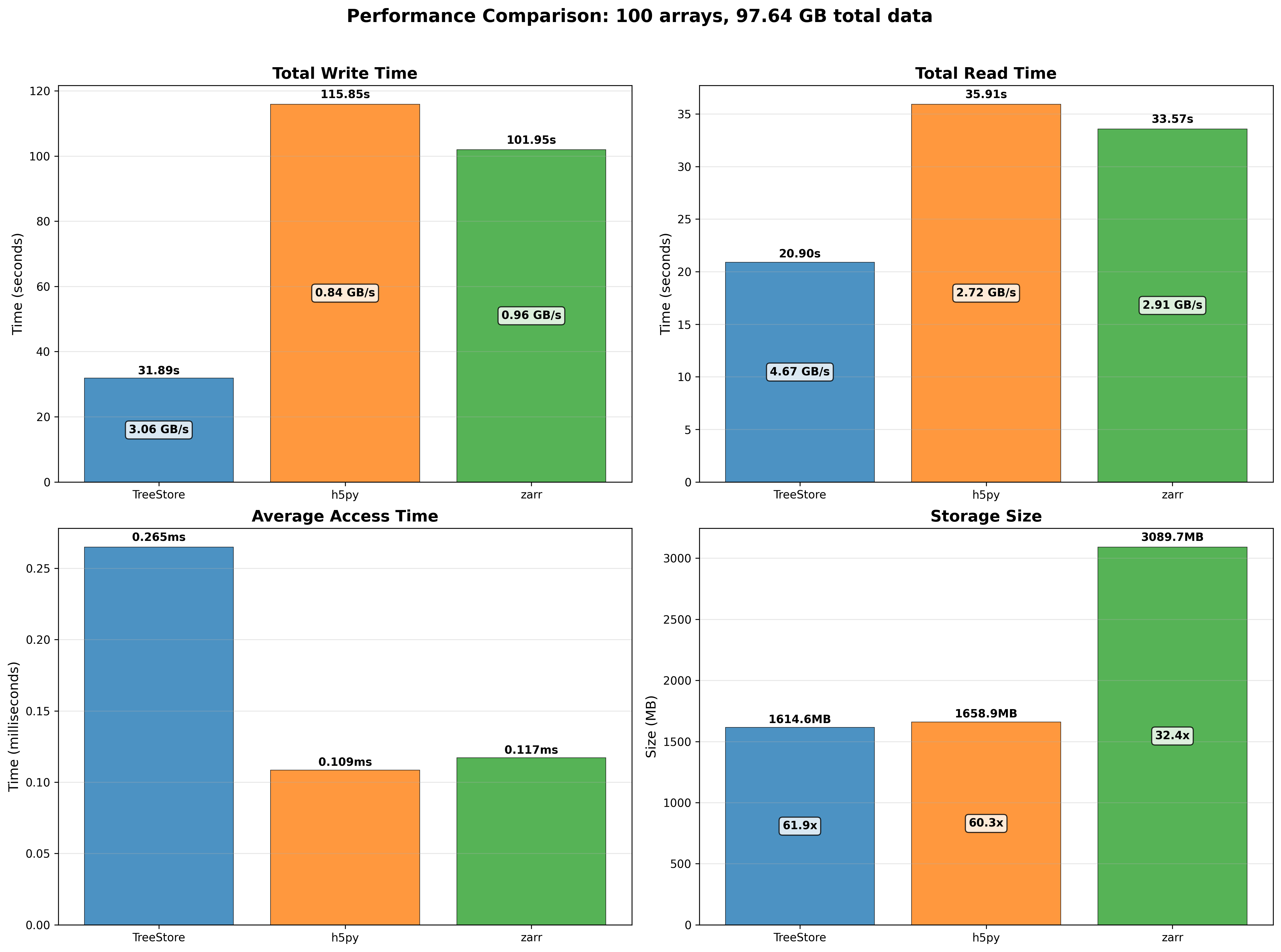
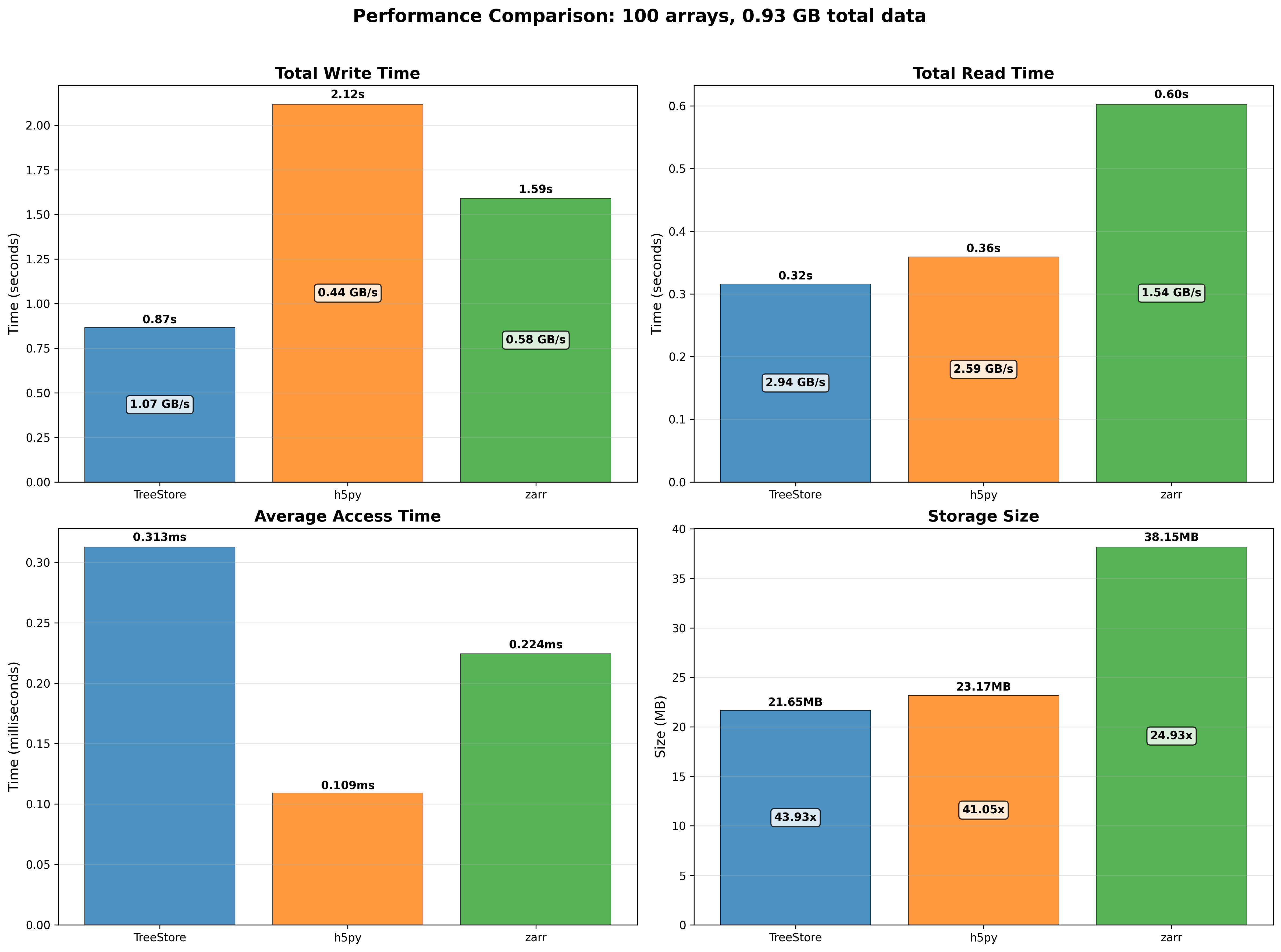
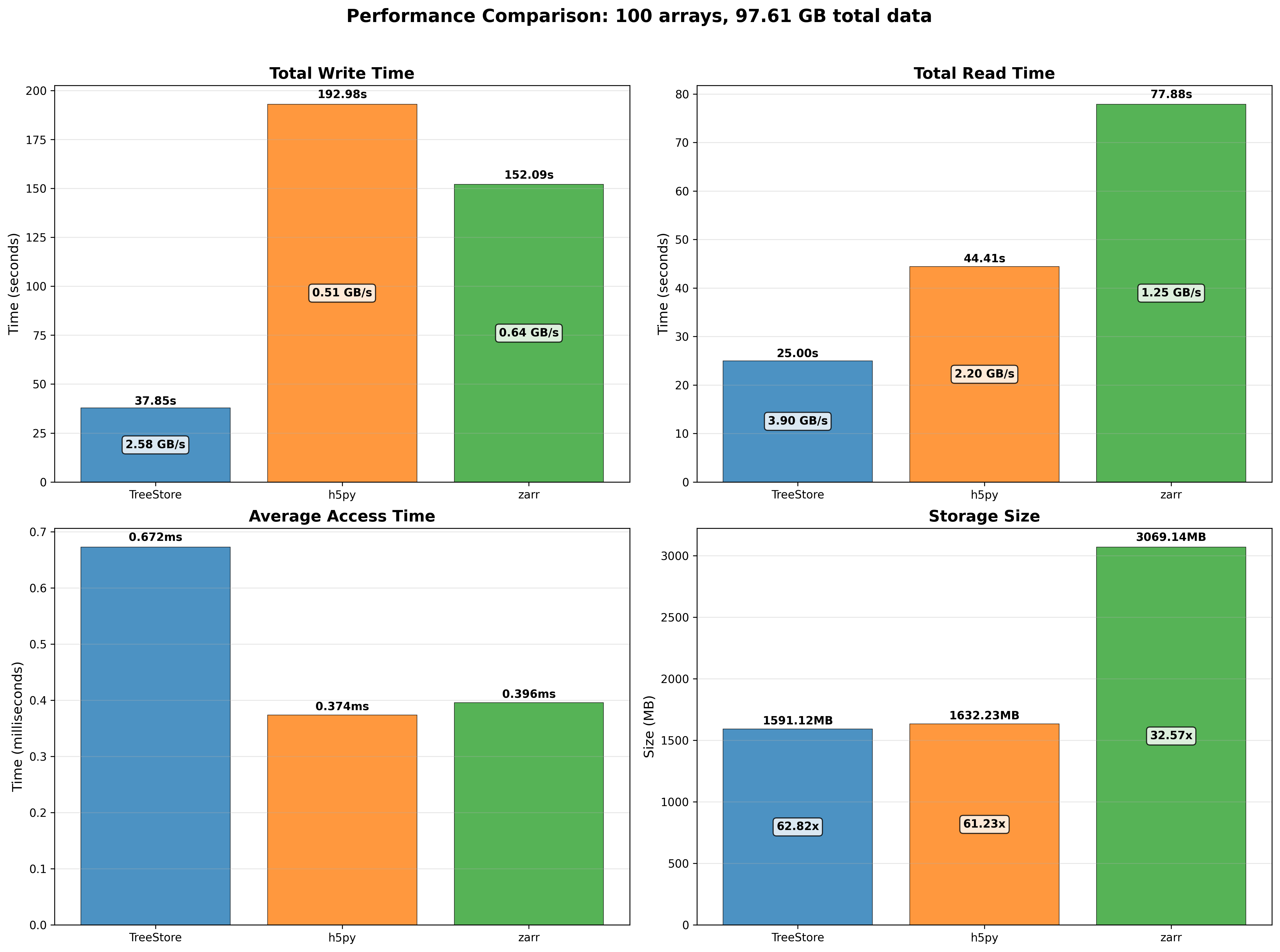
TreeStore is based on powerful abstractions from the blosc2 library, so it is very fast. Here are some benchmarks comparing TreeStore to other data storage formats, like HDF5 and Zarr. We have used two different configurations: one with small arrays, where sizes follow a normal distribution centered at 10 MB each, and the other with larger arrays, where sizes follow a normal distribution centered at 1 GB each. We have compared the performance of TreeStore against HDF5 and Zarr for both small and large arrays, measuring the time taken to create and read datasets. For comparing apples with apples, we have used the same compression codec (zstd) and filter (shuffle) for all three formats.
For assessing different platforms, we have used a desktop with an Intel i9-13900K CPU and 32 GB of RAM, running Ubuntu 25.04, and also a Mac mini with an Apple M4 Pro processor and 24 GB of RAM. The benchmarks were run using this script.
Results for the Intel i9-13900K desktop
100 small arrays (around 10 MB each) scenario:
For the small arrays scenario, we can see that TreeStore is the fastest to create datasets (due to use of multi-threading), but it is slower than HDF5 and Zarr when reading datasets. The reason for this is two-fold: first, TreeStore is designed to work using multi-threading, so it must setup the necessary threads at the beginning of the read operation, which takes some time; second, TreeStore is using NDArray objects internally, which are using a double partitioning scheme (chunks and blocks) to store the data, which adds some overhead when reading small slices of data. Regarding the space used, TreeStore is the most efficient, very close to HDF5, and significantly more efficient than Zarr.
100 large arrays (around 1 GB each) scenario:
When handling larger arrays, TreeStore maintains its lead in creation and full-read performance. Although HDF5 and Zarr offer faster access to small data slices, TreeStore compensates by being the most storage-efficient format, followed by HDF5, with Zarr being the most space-intensive.
Results for the Apple M4 Pro Mac mini
100 small arrays (around 10 MB each) scenario:
100 large arrays (around 1 GB each) scenario:
Consistent with the previous results, TreeStore is the most space-efficient format and the fastest for creating and reading datasets, particularly for larger arrays. Its performance is slower than HDF5 and Zarr only when reading small data slices (access time). This can be improved by reducing the number of threads from the default of eight, which lessens the thread setup overhead. For more details on this, see these slides comparing 8-thread vs 1-thread performance.
Notably, the Apple M4 Pro processor shows competitive performance against the Intel i9-13900K CPU, a high-end desktop processor that consumes up to 8x more power. This result underscores the efficiency of the ARM architecture in general and Apple silicon in particular.
Conclusion
In summary, blosc2.TreeStore offers a straightforward yet potent solution for hierarchically organizing compressed datasets. By merging the high-performance compression of blosc2.NDArray and blosc2.SChunk with a flexible, filesystem-like structure and metadata support, it stands out as an excellent choice for managing complex data projects.
As TreeStore is currently in beta, we welcome feedback and suggestions for its improvement. For further details, please consult the official documentation for blosc2.TreeStore.
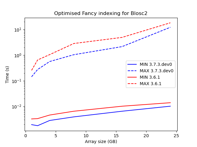
Update (2025-08-26): After some further effort, the 1D fast path mentioned below has been extended to the multidimensional case, with consequent speedups in Blosc2 3.7.3! See below plot comparing maximum and minimum indexing times for the Blosc2-supported fancy indexing cases mentioned below.
---
In response to requests from our users, the Blosc2 team has introduced a fancy indexing capability into the flagship Blosc2 NDArray object. In the future, this could be extended to other classes within the Blosc2 library, such as C2Array and LazyArray.
What is Fancy Indexing?
In many array libraries, most famously NumPy, fancy indexing refers to a vectorized indexing format which allows for simultaneous selection and reshaping of arrays (see this excerpt). For example, one may wish to select three entries from a 1D array:
arr = array([10, 11, 12])
which can be done like so:
arr[[1,2,1]]
>> array([11, 12, 11])
Note that the order of the indices is arbitrary (i.e. the elements of the output may occur in a different order to the original array) and indices may be repeated. Moreover, if the array is multidimensional, for example:
NumPy supports many different kinds of fancy indexing, a flavour of which can be seen from the following examples, where row and col are integer array objects. If they are not of the same shape then broadcasting conventions will be applied to try to massage the index into an understandable format.
arr[row]
arr[[row, col]]
arr[row, col]
arr[row[:, None], col]
arr[1, col] or arr[1:9, col]
In addition, one may use a boolean mask, in combination with integer indices, slices, or integer arrays via
arr[row[:, None], mask]
where the mask must have the same length as the indexed dimension(s).
Support for Fancy Indexing and ndindex
Other libraries for management of large arrays such as zarr and h5py offer fancy indexing support but neither are as comprehensive as NumPy. h5py, which uses the HDF5 format, is quite limited in that one may only use one integer array, no repeated indices are allowed, and the array must be sorted in increasing order, although mixed slice and integer array indexing is possible.
zarr, via its vindex (for vectorized index), offers more support, but is rather limited when it comes to mixed indexing, as slices may not be used with integer arrays, and an integer array must be provided for every dimension of the array (i.e. arr[row] fails on any non-1D arr).
This makes it difficult (in the case of zarr) or impossible (in the case of h5py) to do the kind of reshaping we saw in the introduction (i.e. case 2 above arr[[[1,2],[0,1]]]). This lack of support is due to a combination of: 1) the computational difficulty of many of these operations; and 2) the at times counter-intuitive behaviour of fancy indexing (see the end of this blog post for more details).
When implementing fancy indexing for Blosc2 we strove to match the functionality of NumPy as closely as possible, and we have almost been able to do so — all the 6 cases mentioned above are perfectly feasible with this new Blosc2 release! There are only some minor edge cases which are not supported (see Example 2 in the Addendum). This would not have been possible without the excellent ndindex library, which offers many very useful, efficient functions for index conversion between different shapes and chunks. We can then call NumPy behind-the-scenes, chunk-by-chunk, and exploit its native support for fancy indexing, without having to load the entire array into memory.
Results: Blosc2, Zarr, H5Py and NumPy
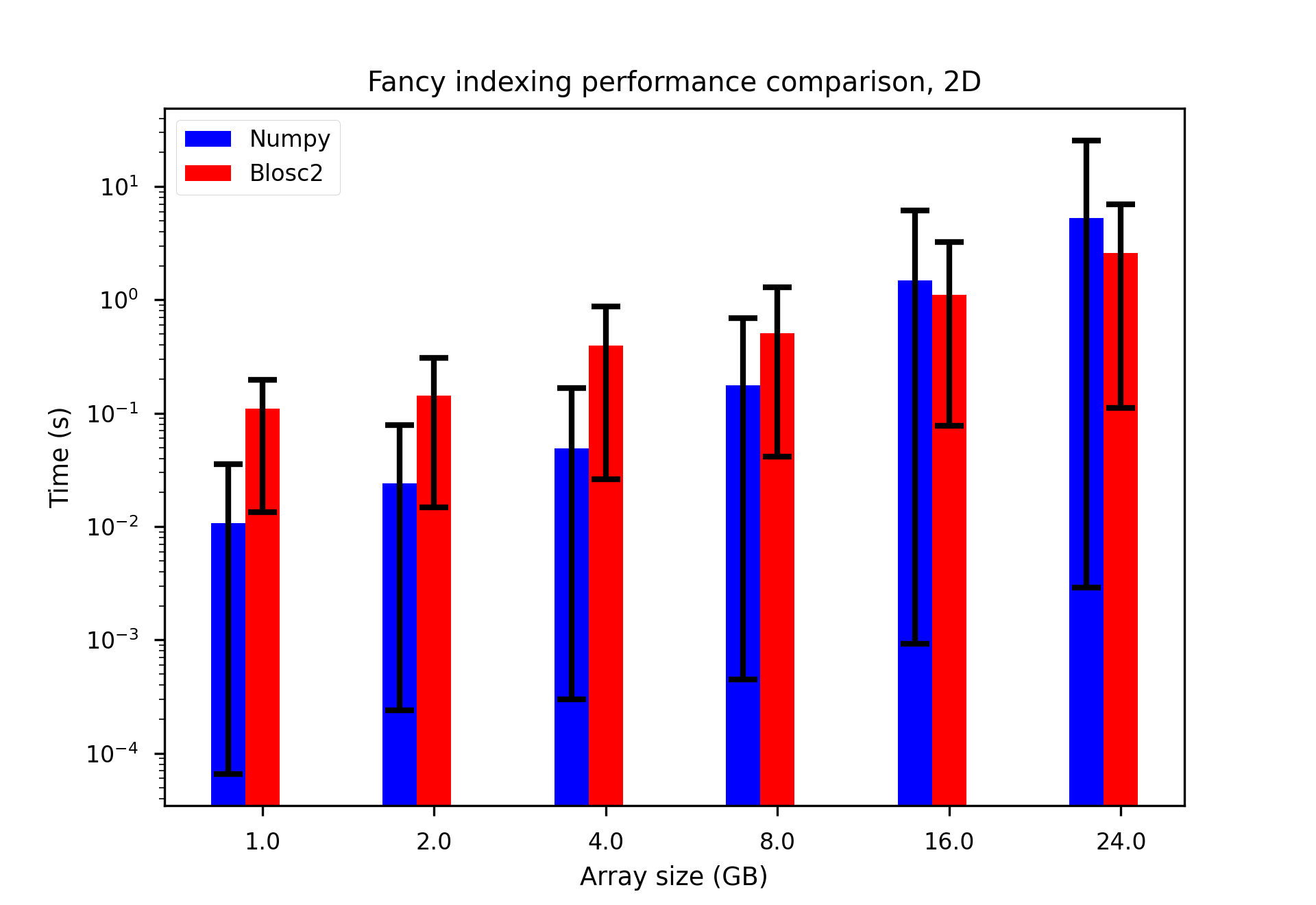
Hence, when averaging over the indexing cases above on 2D arrays of varying sizes, we observe only a minor slowdown for Blosc2 compared to NumPy when the array size is small compared to total memory (24GB), suggesting a small chunking-and-indexing overhead. As expected, when the array grows to an appreciable fraction of memory (16GB), loading the full NumPy array into memory starts to impact performance. The black error bars in the plots indicate the maximum and minimum times observed over the indexing cases (for which there is clearly a large variation).
Note that for cases 4 and 6 with large row or col index arrays, broadcasting causes the resulting index (stored in memory) to be very large, and even for array sizes of 2GB computation is too slow. In the future, we would like to see if this can be improved.
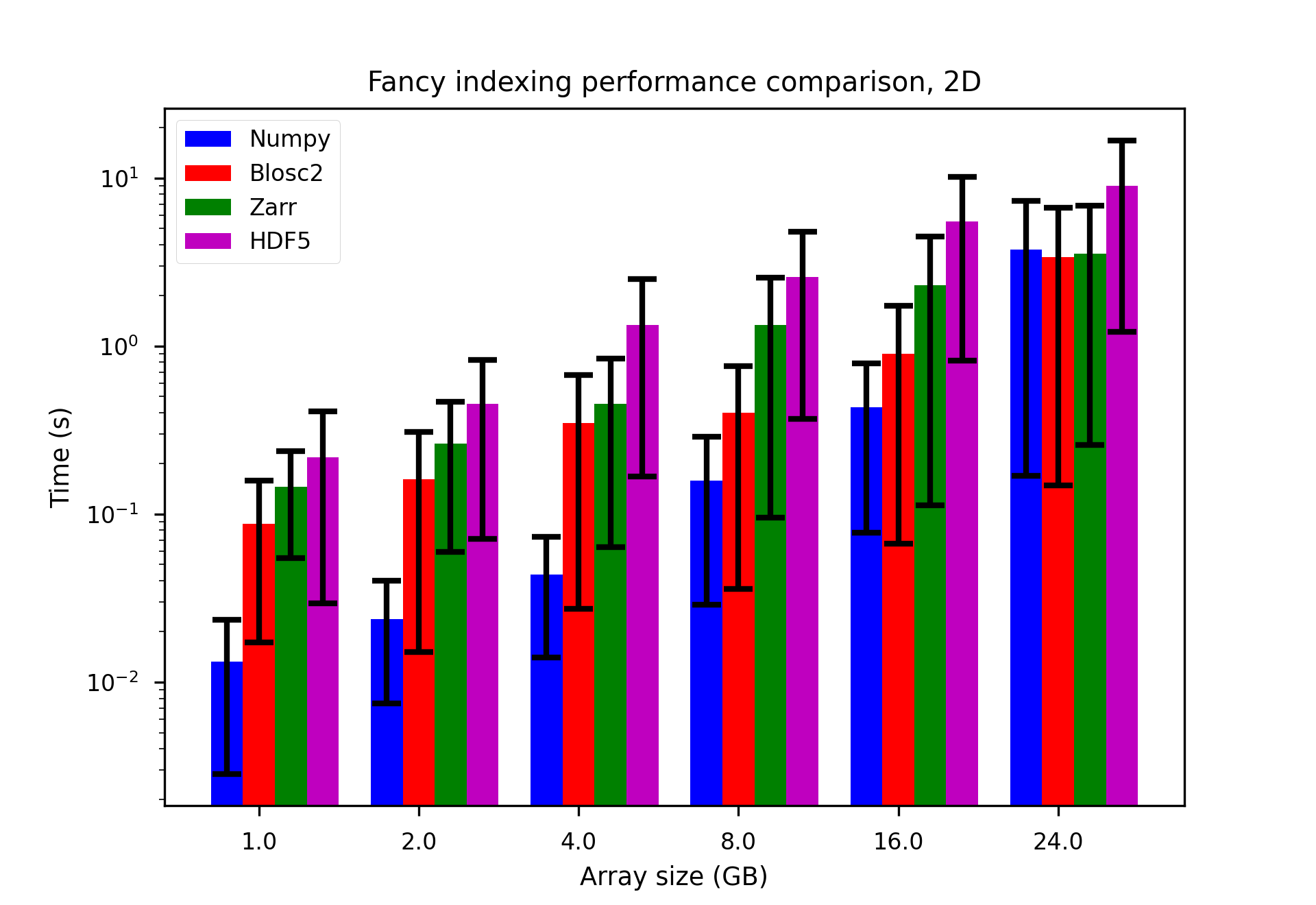
Blosc2 is also as fast or faster than Zarr and HDF5 even for the limited use cases that the latter two libraries both support. HDF5 in particular is especially slow when the indexing array is very large.
These plots have been generated using a Mac mini with the Apple M4 Pro processor. The benchmark is available on the Blosc2 github repo here.
Conclusion
Blosc2 offers a powerful and flexible fancy indexing functionality that is more extensive than that of Zarr and H5Py, while also being able to handle large arrays on-disk without loading them into memory. This makes it a great choice for applications that require complex indexing operations on large datasets.
Give it a try in your own projects! If you have questions, the Blosc2 community is here to help.
If you appreciate what we're doing with Blosc2, please think about supporting us. Your help lets us keep making these tools better.
Addendum: Oindex, Vindex and FancyIndex via Two Examples
Zarr's implementation of fancy indexing is packaged as vindex (vectorized indexing). It also offers another indexing functionality, called orthogonal indexing, via oindex.
The reason for this dual support becomes clear when one considers a simple example.
Example 1
For a 2D array, we have seen that the fancy-indexing rules will cause the two index arrays below to be broadcast together:
arr[[0, 1], [2, 3]] -> [arr[0,2], arr[1,3]]
giving an output with two elements of shape (2,). This is vindexing.
However, one could understand this indexing as selecting rows 0 and 1 in the array, and then their intersection with columns 2 and 3. This gives an output with four elements of shape (2, 2), with elements:
[[arr[0,2], arr[0,3]],
 [arr[1,2], arr[1,3]]]
This is oindexing. Clearly, given the same index, the output is in general different; it is for this reason that the debate about fancy indexing can be quite polemical, and why there is a movement to introduce the vindex/oindex duality in NumPy.
Example 2
I have glossed over this until now, but vindex is not the same as fancy indexing. For this reason Zarr does not support all the functionality of fancy indexing, since it only supports vindex. The most important distinction between the two is that it seeks to avoid certain unexpected fancy indexing behaviour, as can be seen by considering a 3D NumPy array of shape (X, Y, Z) as in the example here. Consider the unexpected behaviour of:
arr[:10, :, [0,1]] has shape (10, Y, 2).

arr[0, :, [0, 1]] has shape (2, Y), not (Y, 2)!!
NumPy indexing treats non-slice indices differently, and will always put the axes introduced by the index array first, unless the non-slice indexes are consecutive, in which case it will try to massage the result to something intuitive (which normally coincides with the result of an oindex) — hence arr[:, 0, [0, 1]] has shape (X, 2), not (2, X).
The hypothesised NumPy vindex would eliminate this transposition behaviour, and be internally consistent, always putting the axes introduced by the index array first. Unfortunately, this is difficult and costly, and so the alternative is to simply not allow such indexing and throw an error, or force the user to be very specific.
Blosc2 will throw an error when one inserts a slice between array indices:
Hopefully you now understand why fancy indexing can be so tricky, and why few libraries seek to support it to the same extent as NumPy - some would say it is perhaps not even desirable to do so!
Update (2025-06-23): Recently, Luke Shaw added a stack() function in Blosc2, using the concatenate feature described here. The new function allows you to stack arrays along a new axis, which is particularly useful for creating higher-dimensional arrays from lower-dimensional ones. We have added a section at the end of this post to show the usage and performance of this new function.
---
Blosc2 just got a cool new trick: super-efficient array concatenation! If you've ever needed to combine several arrays into one, especially when dealing with lots of data, this new feature is for you. It's built to be fast and use as little memory as possible. This is especially true if your array sizes line up nicely with Blosc2's internal "chunks" (think of these as the building blocks of your compressed data). When this alignment happens, concatenation is lightning-fast, making it perfect for demanding tasks.
You can use this new concatenate feature whether you're coding in C or Python, and it works with any Blosc2 NDArray (Blosc2's way of handling multi-dimensional arrays).
Let's see how easy it is to use in Python. If you're familiar with NumPy, the blosc2.concatenate function will feel very similar:
importblosc2# Create some sample arraysa=blosc2.full((10,20),1,urlpath="arrayA.b2nd",mode="w")b=blosc2.full((10,20),2,urlpath="arrayB.b2nd",mode="w")c=blosc2.full((10,20),3,urlpath="arrayC.b2nd",mode="w")# Concatenate the arrays along the first axisresult=blosc2.concat([a,b,c],axis=0,urlpath="destination.b2nd",mode="w")# The result is a new Blosc2 NDArray containing the concatenated dataprint(result.shape)# Output: (30, 20)# You can also concatenate along other axesresult_axis1=blosc2.concat([a,b,c],axis=1,urlpath="destination_axis1.b2nd",mode="w")print(result_axis1.shape)# Output: (10, 60)
The blosc2.concatenate function is pretty straightforward. You give it a list of the arrays you want to join together. You can also tell it which way to join them using the axis parameter (like joining them end-to-end or side-by-side).
A really handy feature is that you can use urlpath and mode to save the combined array directly to a file. This is great when you're working with huge datasets because you don't have to load everything into memory at once. What you get back is a brand new, persistent Blosc2 NDArray with all your data combined.
Aligned versus Non-Aligned Concatenation
Blosc2's concatenate function is smart. It processes your data in small pieces of compressed data (chunks). This has two consequences. The first is that you can join very large arrays, stored on your disk, chunk-by-chunk without using up all your computer's memory. Secondly, if the chunks fit neatly into the arrays to be concatenated, the process is much faster. Why? Because Blosc2 can avoid a lot of extra work, chiefly decompressing and re-compressing the chunks.
Let's look at some pictures to see what "aligned" and "unaligned" concatenation means. "Aligned" means that chunk boundaries of the arrays to be concatenated line up with each other. "Unaligned" means that this is not the case.
The pictures show why "aligned" concatenation is faster. In Blosc2, all data pieces (chunks) inside an array must be the same size. So, if the chunks in the arrays you're joining match up ("aligned"), Blosc2 can combine them very quickly. It doesn't have to rearrange the data into new, same-sized chunks for the final array. This is a big deal for large arrays.
If the arrays are "unaligned," Blosc2 has more work to do. It has to decompress and then re-compress the data to make the new chunks fit, which takes longer. There's one more small detail for this fast method to work: the first array's size needs to be a neat multiple of its chunk size along the direction you're joining.
A big plus with Blosc2 is that it always processes data in these small chunks. This means it can combine enormous arrays without ever needing to load everything into your computer's memory at once.
Performance
To show you how much faster this new concatenate feature is, we did a speed test using LZ4 as the internal compressor in Blosc2. We compared it to the usual way of joining arrays with numpy.concatenate.
The speed tests show that Blosc2's new concatenate is rather slow for small arrays (like 1,000 x 1,000). This is because it has to do a lot of work to set up the concatenation. But when you use larger arrays (like 20,000 x 20,000) that start to exceed the memory limits of our test machine (32 GB of RAM), Blosc2's new concatenate peformance is much better, and nearing the performance of NumPy's concatenate function.
However, if your array sizes line up well with Blosc2's internal chunks ("aligned" arrays), Blosc2 becomes much faster—typically more than 10x times faster than NumPy for large arrays. This is because it can skip a lot of the work of decompressing and re-compressing data, and the cost of copying compressed data is also lower (as much as the achieved compression ratio, which for this case is around 10x).
Using the Zstd compressor with Blosc2 can make joining "aligned" arrays even quicker, since Zstd is good at making data smaller.
So, when arrays are aligned, there's less data to copy (compression ratios here are around 20x), which speeds things up. If arrays aren't aligned, Zstd is a bit slower than the previous compressor (LZ4) because its decompression and re-compression algorithm is slower. Conclusion? Pick the compressor that works best for what you're doing!
Stacking Arrays
We've also added a new stack() function in Blosc2 that uses the concatenate feature. This function lets you stack arrays along a new axis, which is super useful for creating higher-dimensional arrays from lower-dimensional ones. Here's how it works:
importblosc2# Create some sample arraysa=blosc2.full((10,20),1,urlpath="arrayA.b2nd",mode="w")b=blosc2.full((10,20),2,urlpath="arrayB.b2nd",mode="w")c=blosc2.full((10,20),3,urlpath="arrayC.b2nd",mode="w")# Stack the arrays along a new axisstacked_result=blosc2.stack([a,b,c],axis=0,urlpath="stacked_destination.b2nd",mode="w")print(stacked_result.shape)# Output: (3, 10, 20)# You can also stack along other axesstacked_result_axis1=blosc2.stack([a,b,c],axis=1,urlpath="stacked_destination_axis1.b2nd",mode="w")print(stacked_result_axis1.shape)# Output: (10, 3, 20)
Benchmarks for the stack() function show that it performs similarly to the concat() function, especially when the input arrays are aligned. Here are the results for the same data sizes and machine used in the previous benchmarks, and using the LZ4 compressor.
And here are the results for the Zstd compressor.
As can be seen, the stack() function is also very fast when the input arrays are aligned, and it performs well even for large arrays that don't fit into memory. Incidentally, when using the blosc2.stack() function in the last dim, it is slightly faster than numpy.stack() even when the arrays are not aligned; we are not sure why this is the case, but the fact that we can reproduces this behaviour is probably a sign that NumPy can optimize this use case better.
Conclusion
Blosc2's new concatenate and stack features are a great way to combine arrays quickly and without using too much memory. They are especially fast when your array sizes are an exact multiple of Blosc2's "chunks" (aligned arrays), making it perfect for big data jobs. They also work well for large arrays that don't fit into memory, as it processes data in small chunks. Finally, they are supported in both C and Python, so you can use them in your favorite programming language.
Give it a try in your own projects! If you have questions, the Blosc2 community is here to help.
If you appreciate what we're doing with Blosc2, please think about supporting us. Your help lets us keep making these tools better.