Advanced Lazy Expressions and Persistent Reductions

We’re now going to more fully detail Blosc2’s capabilities for lazy computation in Python. In previous tutorials we have hinted at the power of lazy expressions, and in this tutorial we’ll demonstrate exactly how lazy expressions optimize performance by deferring computations. Postponing the computation of the expression until it is actually needed means we can avoid large in-memory temporaries, optimizing memory usage and processing.

However, as mentioned previously, reductions are always computed eagerly when using regular Python expressions with Blosc2 operands. Thus, imprudent use of them could render the lazy expression technique ineffective. Fortunately Blosc2 implements a method to avoid eager computations even when calculating reductions by using a string version of the expression in combination with the blosc2.lazyexpr constructor. We will show how to create and save a lazy expression in this way, and then compute it to obtain the desired results.

We’ll also provide some examples which show how powerful broadcasting can be in Blosc2, and how we can use it to get metadata about the result of a lazy expression without performing the full computation. Access to structural information of the computation result, such as shape and dtype, is hence rapid - even for arbitrarily large arrays. Finally, we’ll demonstrate how such metadata will dynamically adapt to changes in the dimensions and values of the original operands, stored on disk.

Operands as arrays of different shape

We will now create the operands, using a different shape for each of them - remember that this is no problem for Blosc2, which fully supports broadcasting, including for lazy expressions.

import time

import blosc2

# Define dimensions of arrays
dim_a = (200, 300, 400)  # 3D array
dim_b = (200, 400)  # 2D array
dim_c = 400  # 1D array

# Create arrays with specific dimensions and values
a = blosc2.full(dim_a, 1, urlpath="a.b2nd", mode="w")
b = blosc2.full(dim_b, 2, urlpath="b.b2nd", mode="w")
c = blosc2.full(dim_c, 3, urlpath="c.b2nd", mode="w")

Creating and using a string lazy expression

First, let’s build a string expression that sums the contents of array a and performs a multiplication with b and c. In this context, creating a string version of the expression is critical; otherwise, the sum reduction will be computed eagerly.

We may then convert the string to a LazyExpr object using the blosc2.lazyexpr constructor, along with a dictionary which maps the names of the operands within the expression to their corresponding arrays. Since the operands are saved on disk, recall that we can also save the expression to disk.

# Expression that sums all elements of 'a' and multiplies 'b' by 'c'
expression = "a.sum() + b * c"
# Define the operands for the expression
operands = {"a": a, "b": b, "c": c}
# Create a lazy expression
lazy_expression = blosc2.lazyexpr(expression, operands)
# Save the lazy expression to the specified path
url_path = "my_expr.b2nd"
lazy_expression.save(urlpath=url_path, mode="w")

Result Metadata

Note that even though the expression has not been computed, we can access some metadata for the computation result, such as its shape and dtype. On creation, a LazyExpr object uses operand metadata and casting and broadcasting rules to work out some information about the result.

print(f"Result will have shape {lazy_expression.shape} and dtype {lazy_expression.dtype}")

Result will have shape (200, 400) and dtype int64

REFRESHER: Broadcasting allows arrays of different shapes (dimensions) to align for mathematical operations, such as addition or multiplication, without the need to enlarge operands by replicating data. The main idea is that smaller dimensions are “stretched” to larger dimensions in such a way that the operation may be performed consistently.

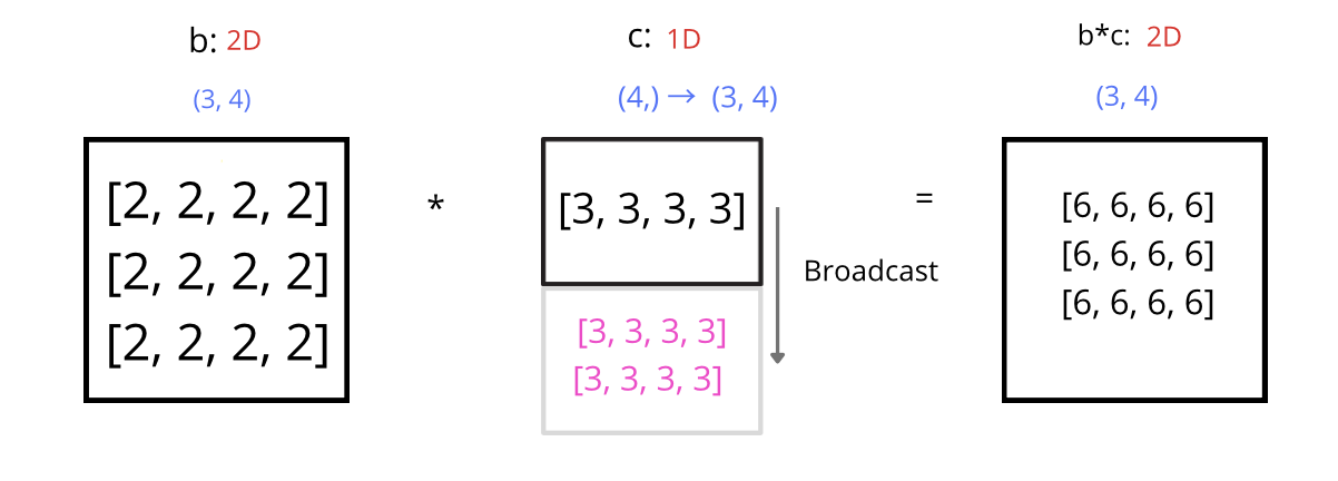
See the NumPy docs on broadcasting for more information.

Computing the lazy expression

Now that we have saved the expression, we can open and compute it to obtain the result. Let’s see how this is done.

lazy_expression = blosc2.open(urlpath=url_path)
# Print the lazy expression and its shape
print(lazy_expression)
t1 = time.time()
print(lazy_expression.shape)
t2 = time.time()
print(f"Time to get shape:{t2 - t1:.5f}")
t1 = time.time()
result1 = lazy_expression.compute()
t2 = time.time()
print(f"Time to compute:{t2 - t1:.5f}")
print("Result of the operation (slice):")
print(result1[:2, :4])  # Print a small slice of the result for demonstration

(o0.sum() + o1 * o2)
(200, 400)
Time to get shape:0.00012
Time to compute:0.09958
Result of the operation (slice):
[[24000006 24000006 24000006 24000006]
 [24000006 24000006 24000006 24000006]]

As we can observe when printing the lazy expression and its shape, the time required to get the shape is significantly shorter than the time to compute the result. This is because lazy_expression.shape does not need to compute all the elements of the expression; instead, it only accesses the metadata of the operands, from which it infers the necessary information about the dimensions and type of the result.

Thanks to this metadata, if we know the dimensions of the arrays involved in the operation (such as in the case of a.sum() + b * c), Blosc2 can quickly infer the resulting shape without performing intensive calculations. This allows for fast access to structural information (like the shape and dtype) without operating on the actual data.

In contrast, when we call lazy_expression.compute(), all the necessary operations to calculate the final result are executed. Here is where the real computation takes place, and as we can see from the time, this process takes longer.

Dynamic adaptation and lazy expressions

In this section, we will see how persisted lazy expressions automatically adapt to changes in the dimensions and values of the original operands, such as the arrays a and b.

# Resizing arrays and updating values to see changes in the expression result
a.resize((300, 300, 400))
a[200:300] = 3
b.resize((300, 400))
b[200:300] = 5
# Open the saved file
lazy_expression = blosc2.open(urlpath=url_path)
t1 = time.time()
print(lazy_expression.shape)
t2 = time.time()
print(f"Time to get shape:{t2 - t1:.5f}")
t1 = time.time()
result2 = lazy_expression.compute()
t2 = time.time()
print(f"Time to compute:{t2 - t1:.5f}")
print("Result of the operation (slice):")
print(result2[:2, :4])

(300, 400)
Time to get shape:0.00020
Time to compute:0.13406
Result of the operation (slice):
[[60000006 60000006 60000006 60000006]
 [60000006 60000006 60000006 60000006]]

After increasing the dimensions of the original arrays by modifying the values of a and b, we reopen the lazy expression (although we do not modify it explicitly). Upon reopening, the lazy expression updates its operand references to refer to the new operand values. From there, we can see that the metadata and final result indeed reflect the changes in the array operands. As before, obtaining the updated structural information (the shape) of the expression is a quick process, since using updated metadata bypasses the need to do the full computation with the new operands (which takes more time).

Note that the dynamic adaptation of lazy expressions to changes in the operands is not limited to the string lazy expression interface; it also works just as well with the Python expression interface we have seen in the other tutorials:

a = blosc2.arange(0, 10, urlpath="a.b2nd", mode="w")
lexpr = a + 1
print(f"Old a: {lexpr[:]}")
a = blosc2.arange(10, 20, urlpath="a.b2nd", mode="w")
print(f"New a: {lexpr[:]}")  # This will still compute the original expression

Old a: [ 1  2  3  4  5  6  7  8  9 10]
New a: [11 12 13 14 15 16 17 18 19 20]

# Clean up the created files
blosc2.remove_urlpath("a.b2nd")
blosc2.remove_urlpath("b.b2nd")
blosc2.remove_urlpath("c.b2nd")
blosc2.remove_urlpath("my_expr.b2nd")

Conclusion

The dynamic adaptation of lazy expressions to changes in the dimensions of array operands illustrates the power of deferred computations in Blosc2. By deferring the computation of expressions until necessary, Blosc2 can quickly access structural information about the result, such as the shape and dtype, even when operands change on disk, without performing intensive calculations. We can also avoid memory-starving temporaries, freeing up resources for the truly necessary computation steps. Broadcasting support also facilitates working with arrays of different sizes offering a powerful and intuitive interface for defining expressions.