What is it?

Python-Blosc2 is a high-performance compressed ndarray library with a flexible compute engine. The compression functionality comes courtesy of the C-Blosc2 library. C-Blosc2 is the next generation of Blosc, an award-winning library that has been around for more than a decade, and that is being used by many projects, including PyTables or Zarr.

Python-Blosc2’s bespoke compute engine allows for complex computations on compressed data, whether the operands are in memory, on disk, or accessed over a network. This capability makes it easier to work with very large datasets, even in distributed environments.

Interacting with the Ecosystem

Python-Blosc2 is designed to integrate seamlessly with existing libraries and tools in the Python ecosystem, including:

• Support for NumPy’s universal functions mechanism, enabling the combination of the NumPy and Blosc2 computation engines.

• Excellent integration with Numba and Cython via User Defined Functions.

• By making use of the simple and open

C-Blosc2 format for storing compressed data, Python-Blosc2 facilitates seamless integration with many other systems and tools.

Python-Blosc2’s compute engine

The compute engine is based on lazy expressions that are evaluated only when needed and can be stored for future use.

Python-Blosc2 leverages both NumPy and NumExpr to achieve high performance, but with key differences. The main distinctions between the new computing engine and NumPy or NumExpr include:

• Support for compressed ndarrays stored in memory, on disk, or over the network.

• Ability to evaluate various mathematical expressions, including reductions, indexing, and filters.

• Support for broadcasting operations, enabling operations on arrays with different shapes.

• Improved adherence to NumPy casting rules compared to NumExpr.

• Support for proxies, facilitating work with compressed data on local or remote machines.

Data Containers

When working with data that is too large to fit in memory, one solution is to load the data in chunks, process each chunk, and then write the results back to disk. If each chunk is compressed, say by a factor of 10, this approach can be especially efficient, since one is essentially able to send the data 10x faster over the network and store it 10x smaller on disk. Even if the data fits in memory, it is often beneficial to use compression and chunking to make more effective use of the cache structure of modern CPUs.

The combined chunking-compression approach is the basis of the main data container objects in Python-Blosc2:

• SChunk: A 64-bit compressed store suitable for any data type supporting the buffer protocol.

• NDArray: An N-Dimensional store that mirrors the NumPy API, enhanced with efficient compressed data storage.

These containers are described in more detail below.

SChunk: a 64-bit compressed store

SChunk is a simple data container that handles setting, expanding and getting data and metadata. A super-chunk is a wrapper around some set of chunked data, and can update and resize the data that it contains, supports user metadata, and has virtually unlimited storage capacity (each constituent chunk of the super-chunk cannot store more than 2 GB). The separate chunks are in general not stored sequentially, which allows for efficient extension of the super-chunk (a new chunk may be inserted anywhere there is space available, and the super-chunk can be extended with a reference to the location of the new chunk).

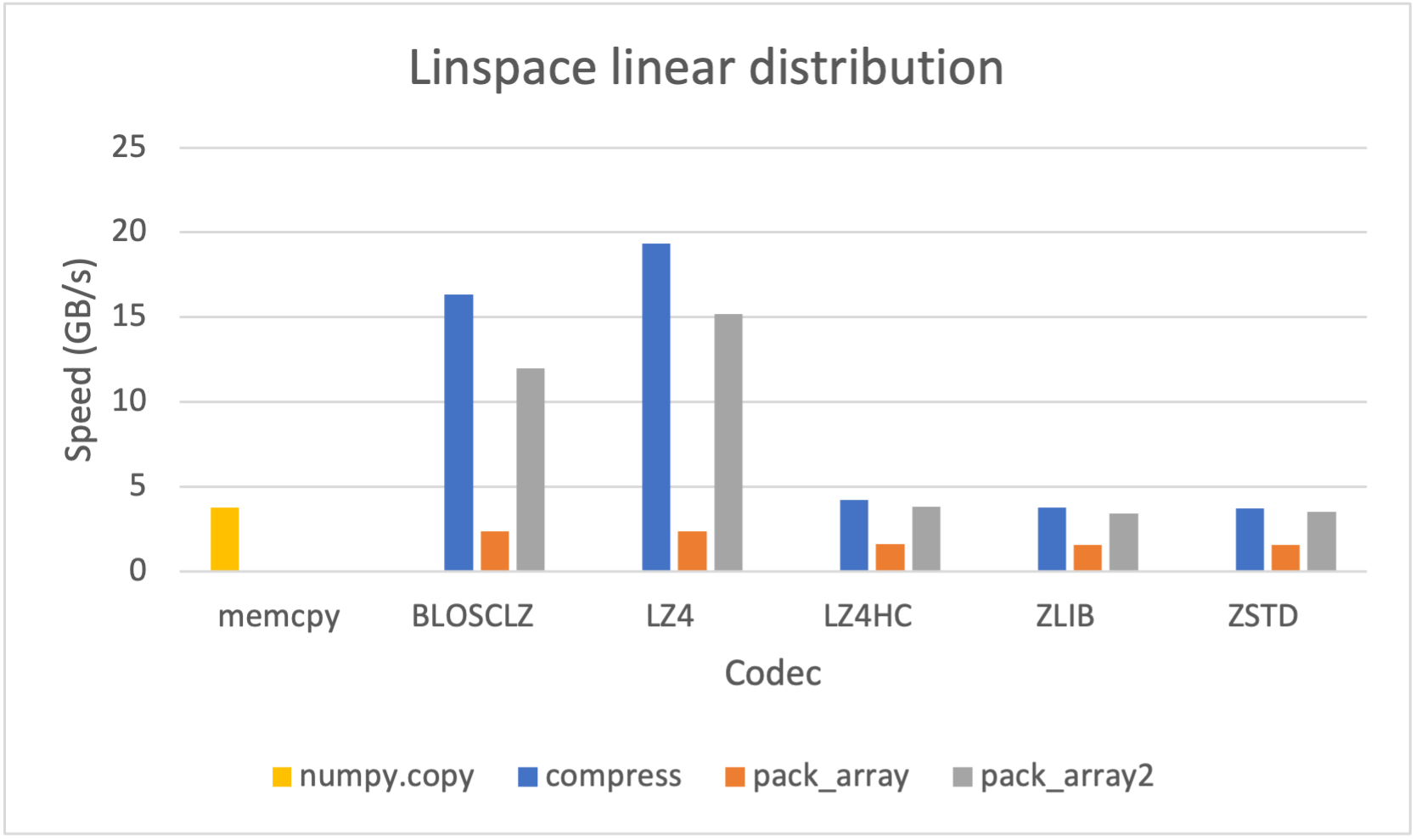
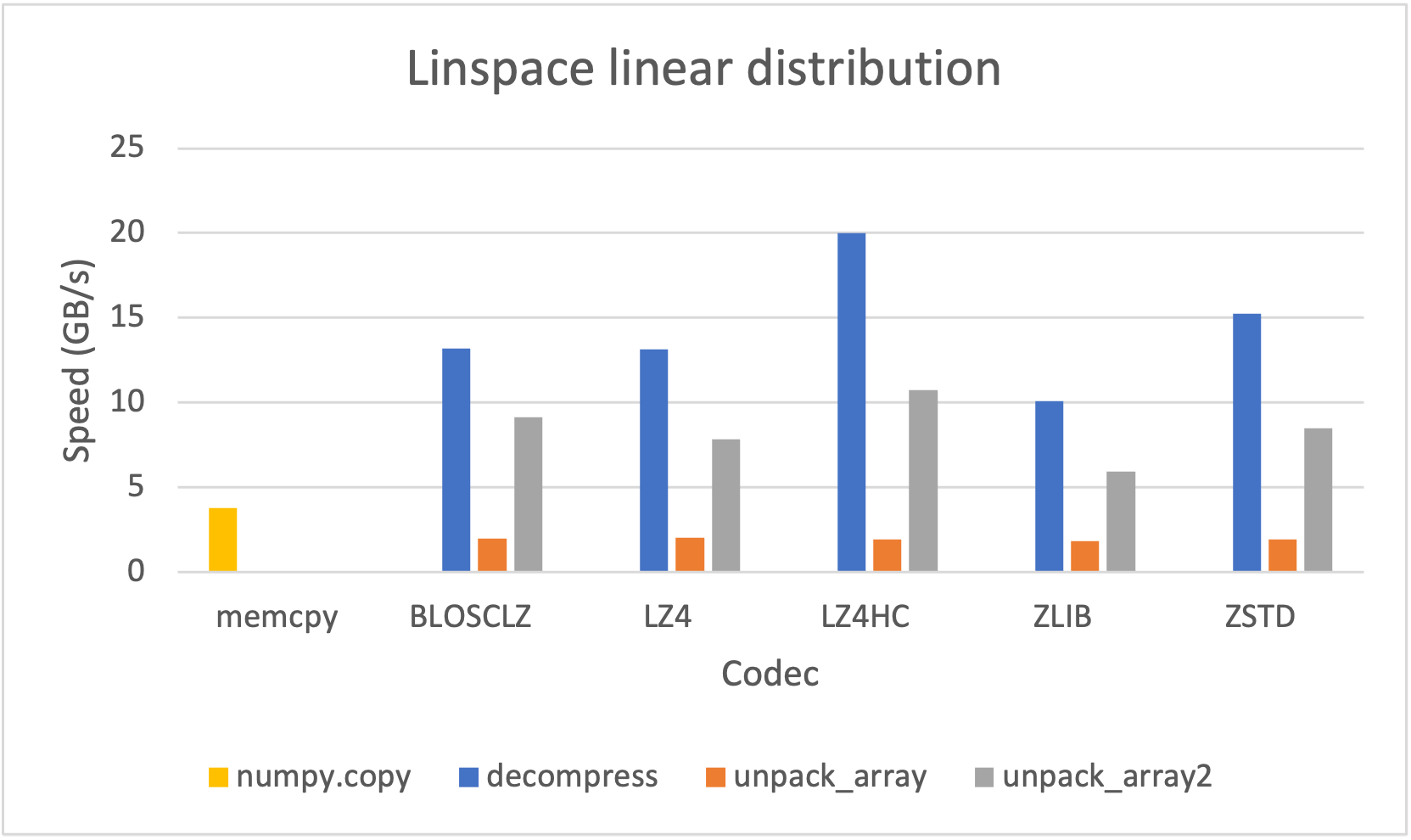
However, since it may be advantageous (for e.g. faster file transfer) to convert a SChunk into a contiguous, serialized buffer (aka cframe), such functionality is supported; likewise one may convert a cframe into a SChunk. The serialization/deserialization process also works with NumPy arrays and PyTorch/TensorFlow tensors at lightning-fast speed:

while reaching excellent compression ratios:

Also, if you are a Mac Silicon owner you may make use of its native arm64 arch, since we distribute Mac arm64 wheels too:

Read more about SChunk features in our blog entry at: https://www.blosc.org/posts/python-blosc2-improvements

NDArray: an N-Dimensional store

A recent feature in Python-Blosc2 is the NDArray object. It rests atop the SChunk object, offering a NumPy-like API for compressed n-dimensional data, with the same chunked storage.

It efficiently reads/writes n-dimensional datasets using an n-dimensional two-level partitioning scheme (each chunk is itself divided into blocks), enabling fine-grained slicing of large, compressed data:

As an example, see how the NDArray object excels at retrieving slices orthogonal to different axes of a 4-dimensional dataset:

More information on chunk-block double partitioning is available in this blog post. Or if you’re a visual learner, see this short video.

Computing with NDArrays

Python-Blosc2’s NDArray objects are designed for ease of use, demonstrated by this example, which closely mirrors the very familiar NumPy syntax:

import blosc2

N = 20_000
# N = 70_000 # for large scenario
a = blosc2.linspace(0, 1, N * N, shape=(N, N))
b = blosc2.linspace(1, 2, N * N, shape=(N, N))
c = blosc2.linspace(-10, 10, N * N, shape=(N, N))
expr = ((a**3 + blosc2.sin(c * 2)) < b) & (c > 0)

out = expr.compute()
print(out.info)

NDArray instances resemble NumPy arrays, since one may expose their shape, dtype etc. via attributes (try a.shape in the example above), but store compressed data, processed efficiently by Python-Blosc2’s engine. This means that you can work with datasets larger than would be feasible with e.g. NumPy.

To see this, we can compare the execution time for the above example (see the benchmark here) when the operands fit in memory uncompressed (20,000 x 20,000). Performance for Blosc2 then matches that of top-tier libraries like NumExpr, and exceeds that of NumPy and Numba, with low memory use via default compression. Even for in-memory computations then, Blosc2 compression can speed up computation via fast codecs and filters, plus efficient CPU cache use.

When the operands are so large that they exceed memory (70,000 x 70,000) unless compressed, one can no longer use NumPy or other uncompressed libraries such as NumExpr. Python-Blosc2’s compression and chunking means the arrays may be stored compressed in memory and then processed chunk-by-chunk; both memory footprint and execution time is greatly reduced compared to Dask+Zarr, which also uses compression (see the benchmark here).

Note: For these plots, we made use of the Blosc2 support for MKL-enabled Numexpr for optimized transcendental functions on Intel compatible CPUs.

Reductions and disk-based computations

Of course, it may be the case that, even compressed, data is still too large to fit in memory. Python-Blosc2’s compute engine is perfectly capable of working with data stored on disk, loading the chunked data efficiently to minimise latency, optimizing calculations on datasets too large for memory. Computation results may also be stored on disk if necessary We can see this at work for reductions, which are 1) computationally demanding, and 2) an important class of operations in data analysis, where we often wish to compute a single value from an array, such as the sum or mean.

Example:

import blosc2

N = 20_000  # for small scenario
# N = 100_000 # for large scenario
a = blosc2.linspace(0, 1, N * N, shape=(N, N), urlpath="a.b2nd", mode="w")
b = blosc2.linspace(1, 2, N * N, shape=(N, N), urlpath="b.b2nd", mode="w")
c = blosc2.linspace(-10, 10, N * N, shape=(N, N))  # small and in-memory
# Expression
expr = np.sum(((a**3 + np.sin(a * 2)) < c) & (b > 0), axis=1)

# Evaluate and get a NDArray as result
out = expr.compute()
print(out.info)

This example computes the sum of a boolean array resulting from an expression, where the operands are on disk, with the result being a 1D array stored in memory (or optionally on disk via the out= parameter in compute() or sum() functions). For a more in-depth look at this example, with performance comparisons, see this blog post.

Hopefully, this overview has provided a good understanding of Python-Blosc2’s capabilities. To begin your journey with Python-Blosc2, proceed to the installation instructions. Then explore the tutorials and reference sections for further information.