New features in Python-Blosc2

Retrieve data with __getitem__ and get_slice

The most general way to store data in Python-Blosc2 is through a SChunk (super-chunk) object. Here the data is split into chunks of the same size. So until now, the only way of working with it was chunk by chunk (see the basics tutorial).

With the new version, you can get general data slices with the handy __getitem__() method without having to mess with chunks manually. The only inconvenience is that this returns a bytes object, which is difficult to read by humans. To overcome this, we have also implemented the get_slice() method; it comes with two optional params: start and stop for selecting the slice you are interested in. Also, you can pass to out any Python object supporting the Buffer Protocol and it will be filled with the data slice. One common example is to pass a NumPy array in the out argument:

out_slice = numpy.empty(chunksize * nchunks, dtype=numpy.int32)
schunk.get_slice(out=out_slice)

We have now the out_slice NumPy array filled with the schunk data. Easy and effective.

Set data with __setitem__

Similarly, if we would like to set data, we had different ways of doing it, e.g. with the update_chunk() or the update_data() methods. But those work, again, chunk by chunk, which was a bummer. That's why we also implemented the convenient __setitem__() method. In a similar way to the get_slice() method, the value to be set can be any Python object supporting the Buffer Protocol. In addition, this method is very flexible because it not only can set the data of an already existing slice of the SChunk, but it also can expand (and update at the same time) it.

To do so, the stop param will set the new number of items in SChunk:

start = schunk_nelems - 123
stop = start + new_value.size   # new number of items
schunk[start:stop] = new_value

In the code above, the data between start and the SChunk current size will be updated and then, the data between the previous SChunk size and the new stop will be appended automatically for you. This is very handy indeed (note that the step parameter is not yet supported though).

Serialize SChunk from/to a contiguous compressed buffer

Super-chunks can be serialized in two slightly different format frames: contiguous and sparse. A contiguous frame (aka cframe) serializes the whole super-chunk data and metadata into a sequential buffer, whereas the sparse frame (aka sframe) uses a contiguous frame for metadata and the data is stored separately in so-called chunks. Here it is how they look like:

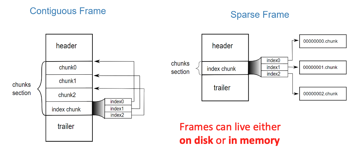
The contiguous and sparse formats come with its own pros and cons. A contiguous frame is ideal for transmitting / storing data as a whole buffer / file, while the sparse one is better suited to act as a store while a super-chunk is being built.

In this new version of Python-Blosc2 we have added a method to convert from a SChunk to a contiguous, serialized buffer:

buf = schunk.to_cframe()

as well as a function to build back a SChunk instance from that buffer:

schunk = schunk_from_cframe(buf)

This allows for a nice way to serialize / deserialize super-chunks for transmission / storage purposes. Also, and for performance reasons, and for reducing memory usage to a maximum, these functions avoid copies as much as possible. For example, the schunk_from_cframe function can build a SChunk instance without copying the data in cframe. Such a capability makes the use of cframes very desirable whenever you have to transmit and re-create data from one machine to another in a very efficient way.

Serializing NumPy arrays

Last but not least, you can also serialize NumPy arrays with the new pair of functions pack_array2() / unpack_array2(). Although you could already do this with the existing pack_array() / unpack_array() functions, the new ones are much faster and do not have the 2 GB size limitation. To prove this, let's see its performance by looking at some benchmark results obtained with an Intel box (i9-10940X CPU @ 3.30GHz, 14 cores) running Ubuntu 22.04.

In this benchmark we are comparing a plain NumPy array copy against compression/decompression through different compressors and functions (compress() / decompress(), pack_array() / unpack_array() and pack_array2() / unpack_array2()). The data distribution for the plots below is for 3 different data distributions: arange, linspace and random:

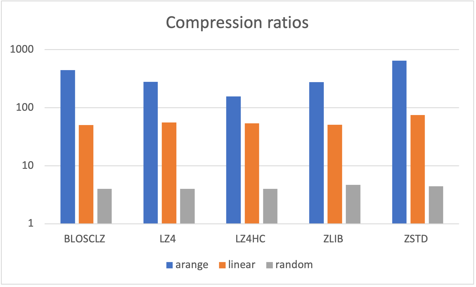
As can be seen, different codecs offer different compression ratios for the different distributions. Note in particular how linear distributions (arange for int64 and linspace for float64) can reach really high compression ratios (very low entropy).

Let's see the speed for compression / decompression; in order to not show too many info in this blog, we will show just the plots for the linspace linear distribution:

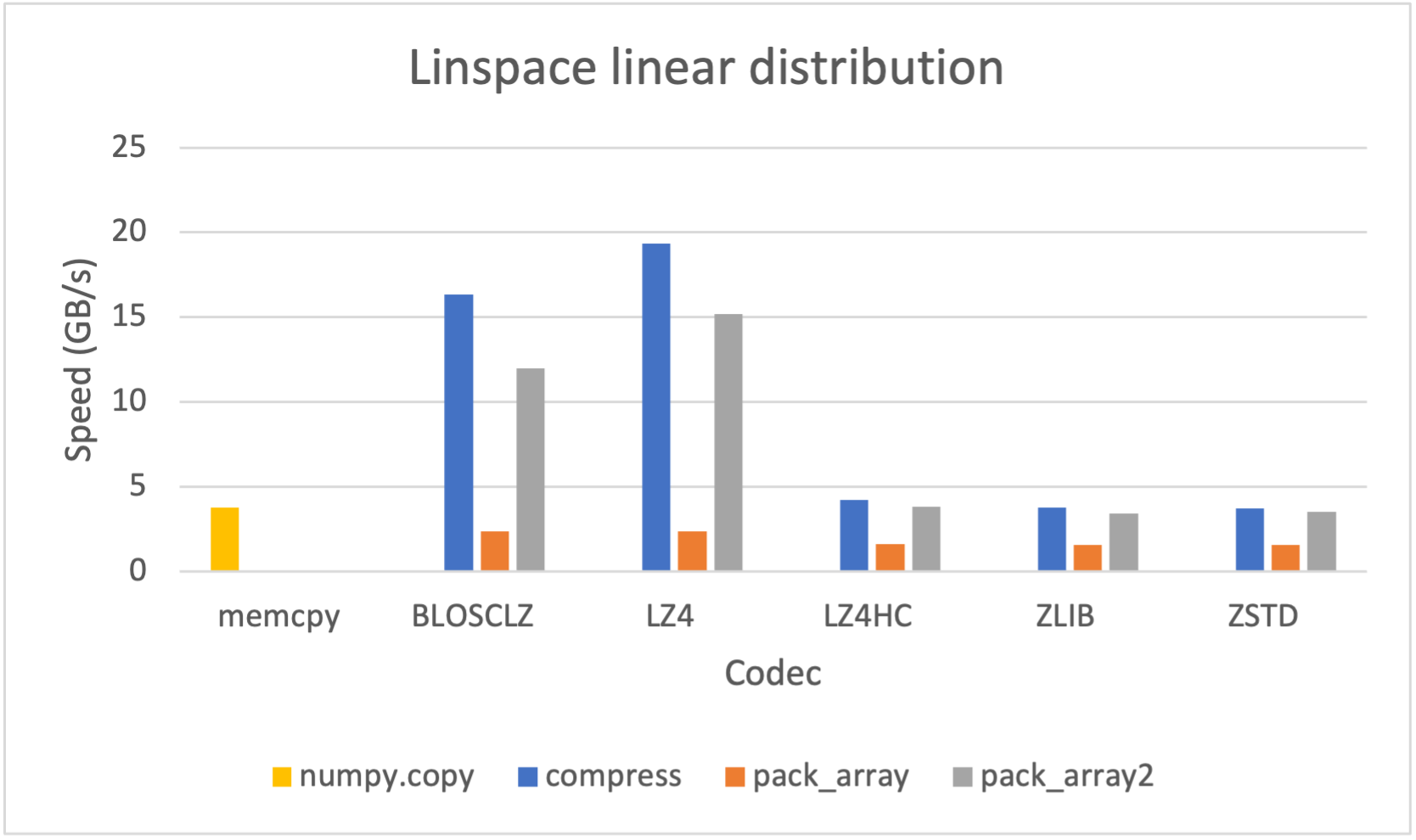
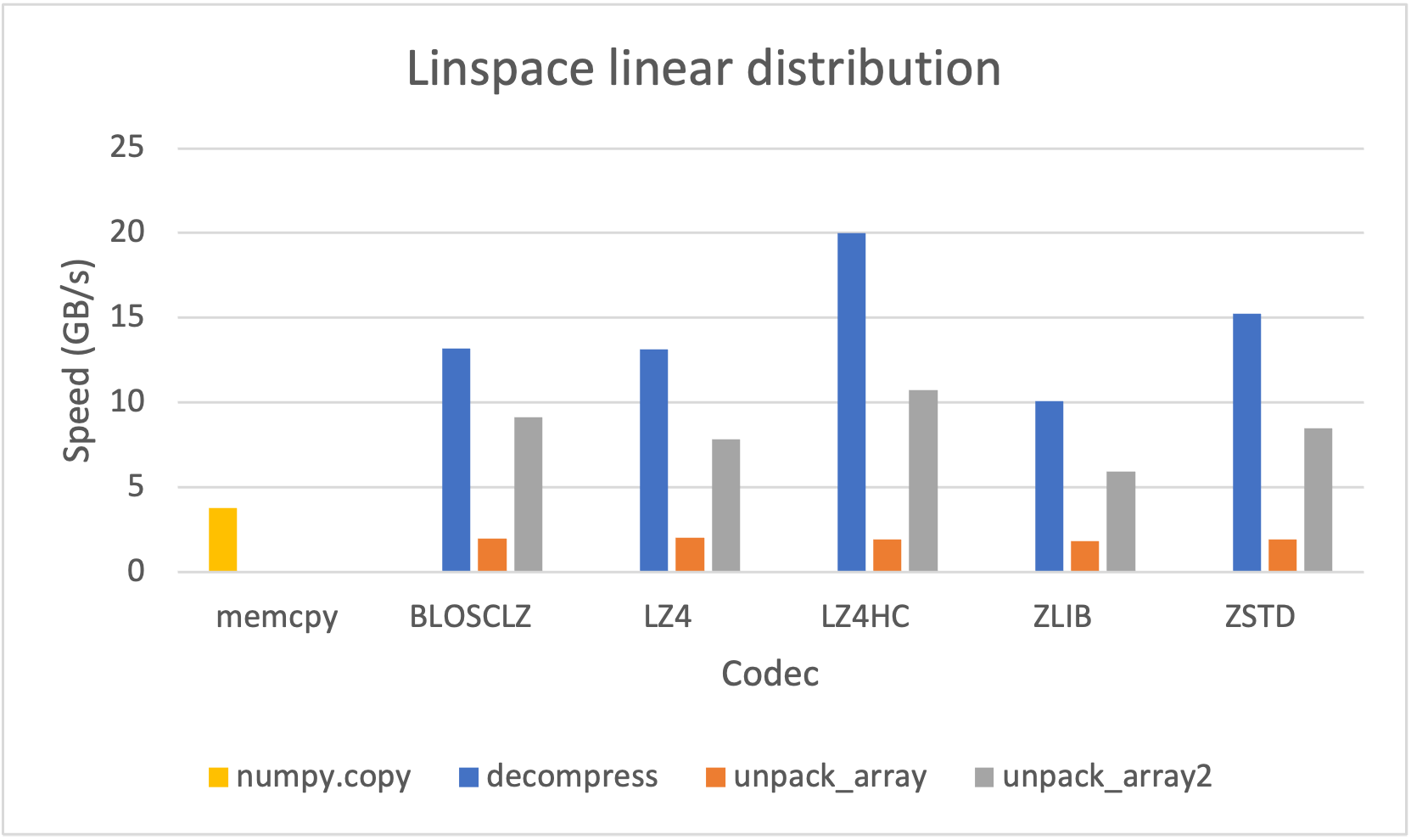
Here we can see that the pair pack_array2() / unpack_array2() is consistently (much) faster than their previous version pack_array() / unpack_array(). Despite that, the fastest is the compress() / decompress() pair; however this is not serializing all the properties of a NumPy array, and has the limitation of not being able to compress data larger than 2 GB.

You can test the speed in your box by running the pack_compress bench.

Also, if you would like to store the contiguous buffer on-disk, you can directly use the pair of functions save_array(), load_array().

Native performance on Apple M1 processors

Contrariliy to Blosc1, Blosc2 comes with native support for ARM processors (it leverages the NEON SIMD instruction set there), and that means that it runs very fast in this architecture. As an example, let's see how the new pack_array2() / unpack_array2() works in an Apple M1 laptop (Macbook Air).

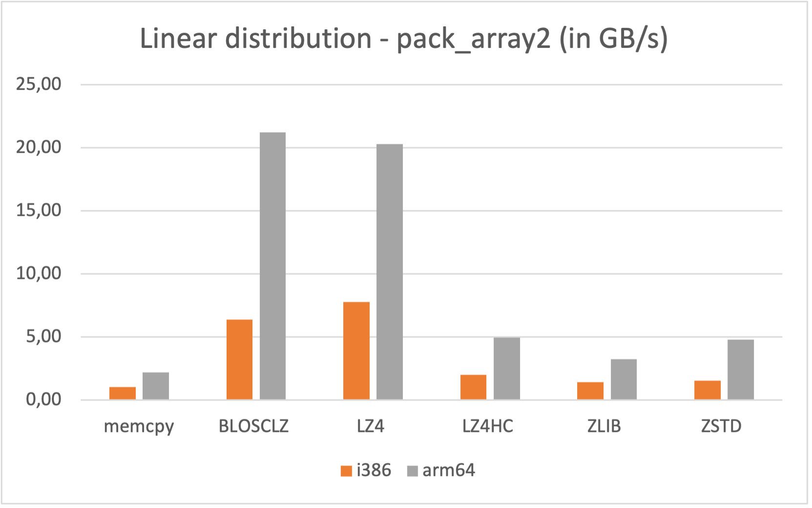
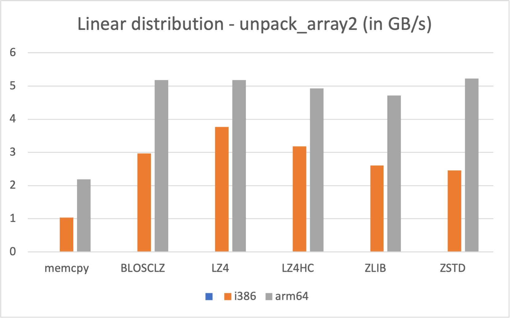
As can be seen, running Blosc2 in native arm64 mode on M1 offers quite a bit more performance (specially during compression) than using the i386 emulation. If speed is important to you, and you have a M1/M2 processor, make sure that you are running Blosc2 in native mode (arm64).

Conclusions

The new features added to python-blosc2 offer an easy way of creating, getting, setting and expanding data by using a SChunk instance. Furthermore, you can get a contiguous compressed representation (aka cframe) of it and re-create it again latter. And you can do the same with NumPy arrays (either in-memory or on-disk) faster than with the former functions, and even faster than a plain memcpy().

For more info on how to use these useful new features, see this Jupyter notebook tutorial.

Finally, the complete documentation is at: https://www.blosc.org/python-blosc2/python-blosc2.html. Thanks to Marc Garcia (@datapythonista) for his fine work and enthusiasm in helping us in providing a better structure to the Blosc documentation!

This work has been possible thanks to a Small Development Grant from NumFOCUS. NumFOCUS is a non-profit organization supporting open code for better science. If you like the goal, consider giving a donation to NumFOCUS (you can optionally make it go to our project too, to which we would be very grateful indeed :-).