N-dimensional reductions with Blosc2
NumPy is widely recognized for its ability to perform efficient computations and manipulations on multidimensional arrays. This library is fundamental for many aspects of data analysis and science due to its speed and flexibility in handling numerical data. However, when datasets reach considerable sizes, working with uncompressed data can result in prolonged access times and intensive memory usage, which can negatively impact overall performance.
Python-Blosc2 leverages the power of NumPy to perform reductions on compressed multidimensional arrays. But, by compressing data with Blosc2, it is possible to reduce the memory and storage space required to store large datasets, while maintaining fast reduction times. This is especially beneficial for systems with memory constraints, as it allows for faster data access and operation.
In this blog, we will explore how Python-Blosc2 can perform data reductions with in-memory NDArray objects (or any other object fulfilling the LazyArray interface) and how the speed of these operations can be optimized by using different chunk shapes, compression levels and codecs. We will then compare the performance of Python-Blosc2 with NumPy.
Note: The code snippets shown in this blog are part of a Jupyter notebook that you can run on your own machine. For that, you will need to install a recent version of Python-Blosc2: pip install 'blosc2>=3.0.0b3'; feel free to experiment with different parameters and share your results with us!
The 3D array
We will use a 3D array of type float64 with shape (1000, 1000, 1000). This array will be filled with values from 0 to 1000, and the goal will be to compute the sum of values in stripes of 100 elements in one axis, and including all the values in the other axis. We will perform reductions along the X, Y, and Z axes, comparing Blosc2 performance (with and without compression) against NumPy.
Reducing with NumPy
We will start by performing different sum reductions using NumPy. First, summing along the X, Y, and Z axes (and getting 2D arrays as result) and then summing along all axis (and getting an scalar as result).
Reducing with Blosc2
Now let's create the Blosc2 array from the NumPy array. First, let's define the parameters for Blosc2: number of threads, compression levels, codecs, and chunk sizes. We will exercise different combinations of these parameters (including no compression) to evaluate the performance of Python-Blosc2 in reducing data in 3D arrays.
The function shown below is responsible for creating the different arrays and performing the reductions for each combination of parameters.
# Create a 3D array of type float64
def measure_blosc2(chunks):
    meas = {}
    for codec in codecs:
        meas[codec] = {}
        for clevel in clevels:
            meas[codec][clevel] = {"sum": {}, "time": {}}
            cparams = {"clevel": clevel, "codec": codec}
            a1 = blosc2.asarray(a, chunks=chunks, cparams=cparams)
            if clevel > 0:
                print(f"cratio for {codec.name} + SHUFFLE: {a1.schunk.cratio:.1f}x")
            # Iterate on Blosc2 and NumPy arrays
            for n, axis in enumerate(axes):
                n = n if axis != "all" else None
                t0 = time()
                # Perform the sum of the stripe (defined by the slice_)
                meas[codec][clevel]["sum"][axis] = a1.sum(axis=n)
                t = time() - t0
                meas[codec][clevel]["time"][axis] = t
                # If interested, you can uncomment the following line to check the results
                #np.testing.assert_allclose(meas[codec][clevel]["sum"][axis],
                #                           meas_np["sum"][axis])
    return meas
Automatic chunking
Let's plot the results for the X, Y, and Z axes, comparing the performance of Python-Blosc2 with different configurations against NumPy.
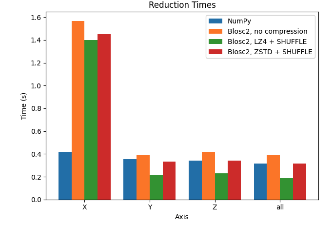
We can see that reduction along the X axis is much slower than those along the Y and Z axis for the Blosc2 case. This is because the automatically computed chunk shape is (1, 1000, 1000) making the overhead of partial sums larger. In addition, we see that, with the exception of the X axis, Blosc2+LZ4+SHUFFLE actually achieves far better performance than NumPy. Finally, when not using compression inside Blosc2, we never see an advantage. See later for a discussion on these results.
Manual chunking
Let's try to improve the performance by manually setting the chunk size. In the next case, we want to make performance similar along the three axes, so we will set the chunk size to (100, 100, 100) (8 MB).
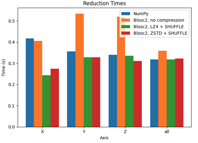
In this case, performance in the X axis is already faster than Y and Z axes for Blosc2. Interestingly, performance is also faster than NumPy in X axis, while being very similar in Y and Z axis.
We could proceed further and try to fine tune the chunk size to get even better performance, but this is out of the scope of this blog (and more a task for Btune). Instead, we will try to make some sense on the results above; see below.
Why Blosc2 can be faster than NumPy?
As Blosc2 is using the NumPy machinery for computing reductions behind the scenes, why is Blosc2 faster than NumPy in several cases above? The answer lies in the way Blosc2 and NumPy access data in memory.
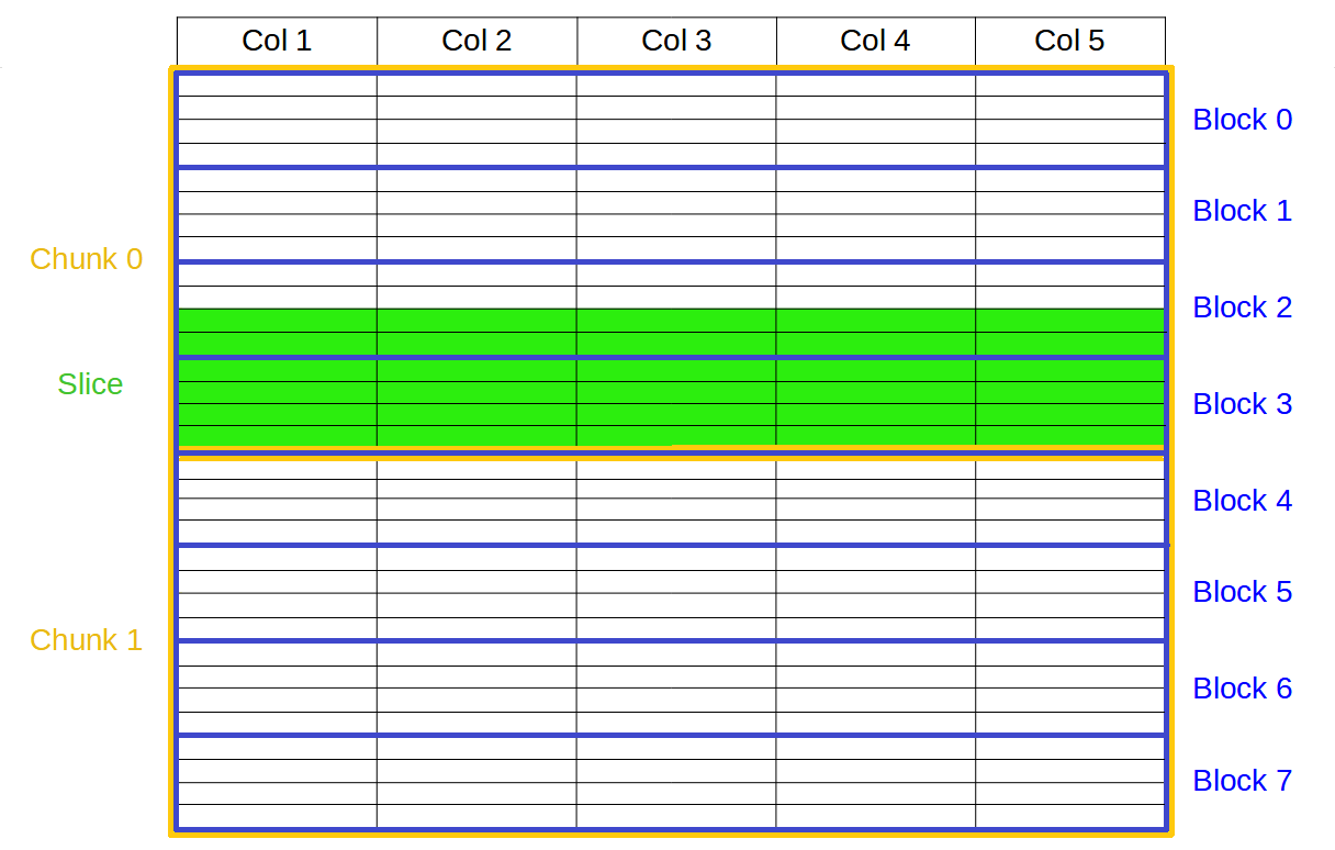
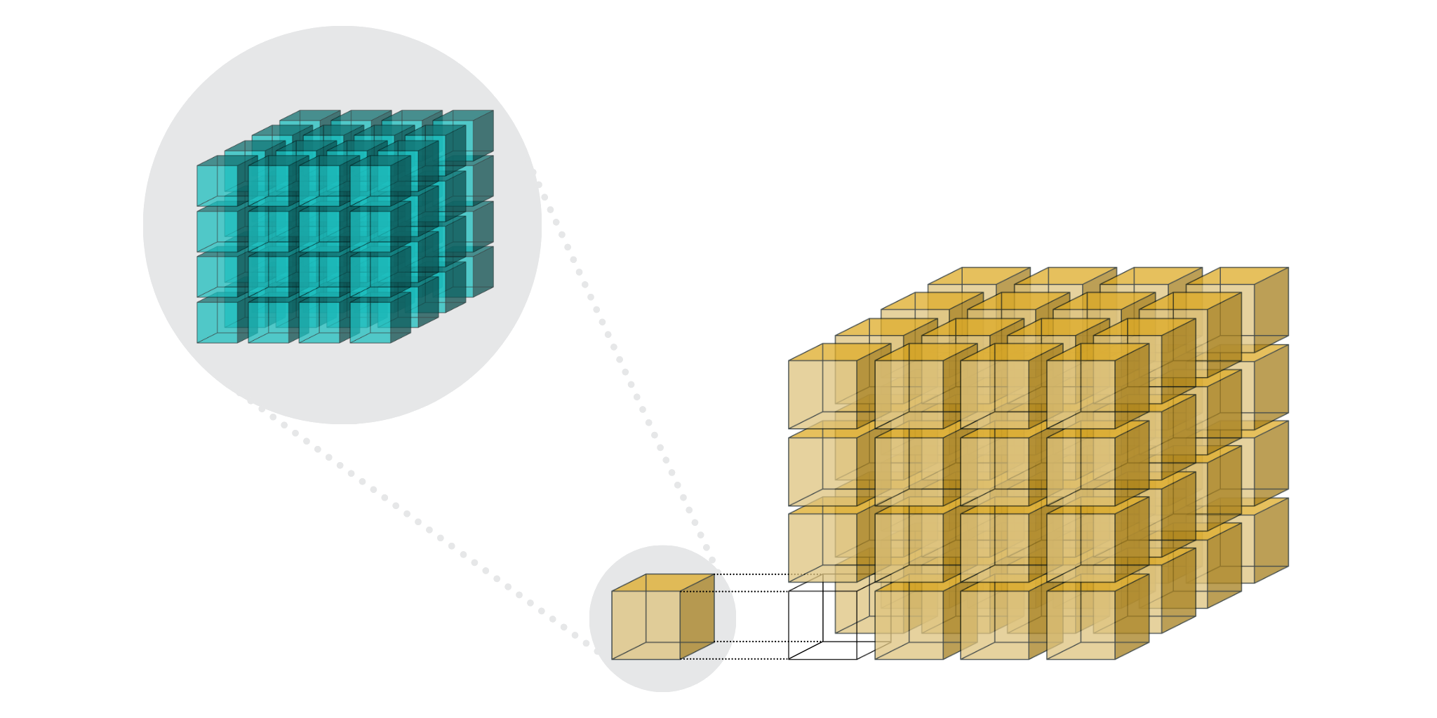
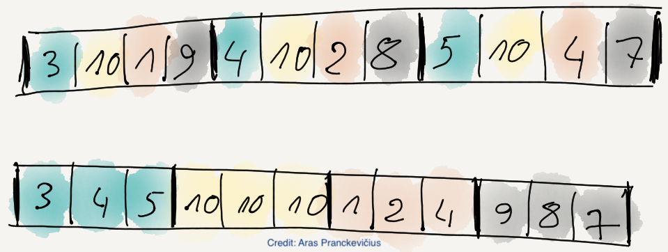
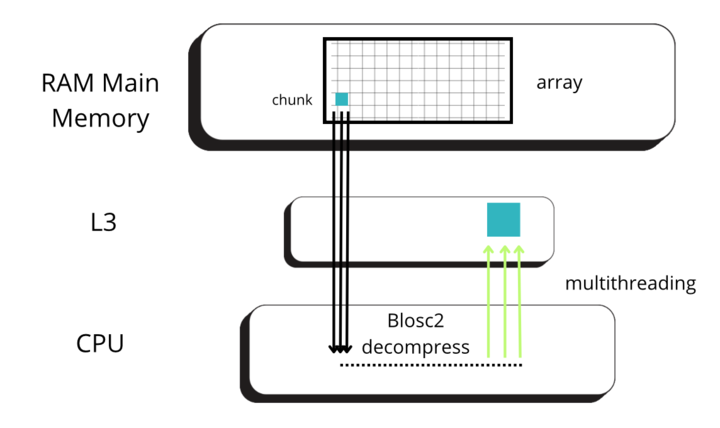
Blosc2 splits data into chunks and blocks to compress and decompress data efficiently. When accessing data, a full chunk is fetched from memory and decompressed by the CPU (as seen in the image below, left side). If the chunk size is small enough to fit in the CPU cache, the CPU can write the decompressed chunk faster, as it does not need to travel back to the main memory. Later, when NumPy is called to perform the reduction on the decompressed chunk, it can access the data faster, as it is already in the CPU cache (image below, right side).
 |
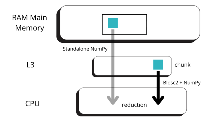 |
But for allowing NumPy go faster, Blosc2 needs to decompress several chunks prior to NumPy performing the reduction operation. The decompressed chunks are stored on a queue, waiting for further processing; this is why Blosc2 needs to handle several (3 or 4) chunks simultaneously. In our case, the L3 cache size of our CPU (Intel 13900K) is 36 MB, and Blosc2 has chosen 8 MB for the chunk size, allowing to store up to 4 chunks in L3, which is near to optimal. Also, when we have chosen the chunk size to be (100, 100, 100), the chunk size is still 8 MB, which continues to be fine indeed.
All in all, it is not that Blosc2 is faster than NumPy, but rather that it is allowing NumPy to leverage the CPU cache more efficiently. Having said this, we still need some explanation on why the performance can be so different along the X, Y, and Z axes, specially for the first chunk shape (automatic) above. Let's address this in the next section.
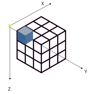
Performing reductions on 3D arrays
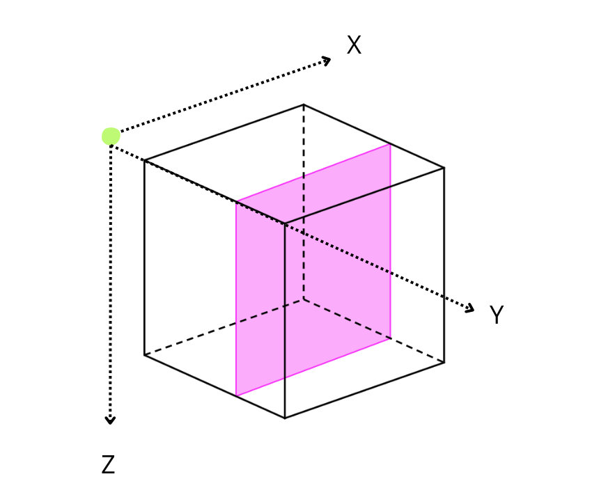
On a three-dimensional environment, like the one shown in the image, data is organized in a cubic space with three axes: X, Y, and Z. By default, Blosc2 chooses the chunk size so that it fits in the CPU cache comfortably. On the other hand, it tries to follow the NumPy convention of storing data row-wise; so, this is why the default chunk shape has been chosen as (1, 1000, 1000). In this case, it is clear that reduction times along different axes are not going to be the same, as the sizes of the chunk in different axes are not uniform (actually, there is a large asymmetry).
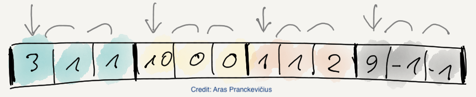
The difference in cost while traversing data values can be visualized more easily on a 2D array:
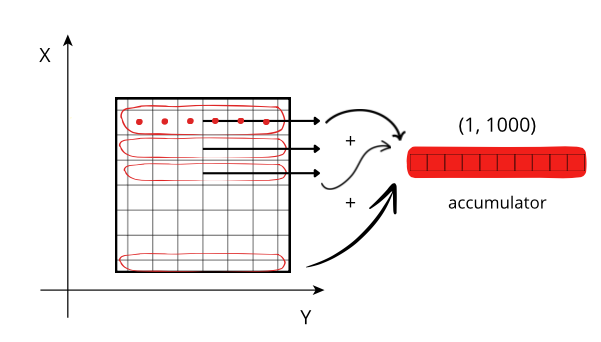
Reduction along the X axis: When accessing a row (red line), the CPU can access these values (red points) from memory sequentially, but they need to be stored on an accumulator. The next rows needs to be fetched from memory and be added to the accumulator. If the size of the accumulator is large (in this case is 1000 * 1000 * 8 = 8 MB), it does not fit in low level CPU caches, and has to be peformed in the relatively slow L3.
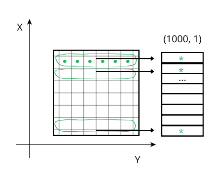
Reducing along the Y axis: When accessing a row (green line), the CPU can access these values (green points) from memory sequentially but, contrarily to the case above, they don't even need an accumulator, and the sum of the row (marked as an *) is final. So, although the number of sum operations is the same as above, the required time is smaller because there is no need of updating all the values of the accumulator per row, but only one at a time, which is faster in modern CPUs.
Tweaking the chunk size
However, when Blosc2 is instructed to create chunks that are the same size for all the axes (chunks=(100, 100, 100)), the situation changes. In this case, an accumulator is needed for each chunk (sub-cube in figure above), but as it is relatively small (100 * 100 * 8 = 80 KB), and fits in L2, so accumulation in the X axis is faster than in the previous scenario (remember that it needs to do the accumulation in L3).
Incidentally, now Blosc2 performance along X axis is even better than in the Y and Z axes, as the CPU can access data in a more efficient way. Furthermore, Blosc2 performance is up to 1.5x better than NumPy in the X axis (while being similar, or even a bit better along Y and Z axes), which is a quite remarkable feat.
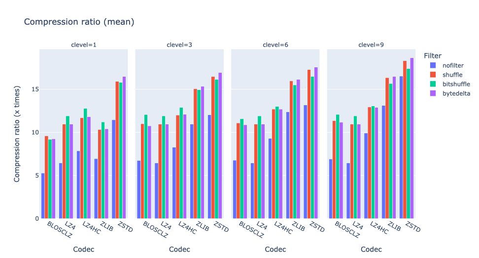
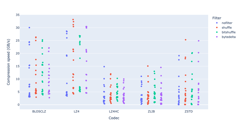
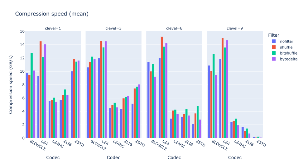
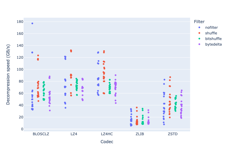
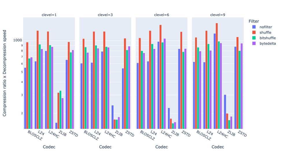
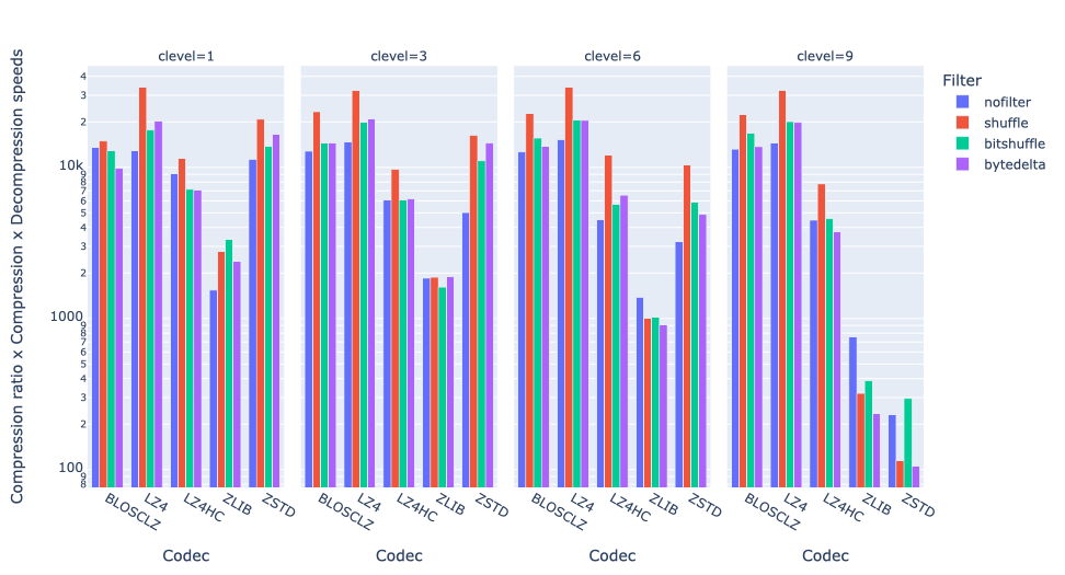
Effect of using different codecs in Python-Blosc2
Compression and decompression consume CPU and memory resources. Differentiating between various codecs and configurations allows for evaluating how each option impacts the use of these resources, helping to choose the most efficient option for the operating environment. Finding the right balance between compression ratio and speed is crucial for optimizing performance.
In the plots above, we can see how using the LZ4 codec is striking such a balance, as it achieves the best performance in general, even above a non-compressed scenario. This is because LZ4 is tuned towards speed, and the time to compress and decompress the data is very low. On the other hand, ZSTD is a codec that is optimized for compression ratio (although not shown, in this case it typically compresses between 2x and 3x more than LZ4), and hence it is a bit slower. However, it is still faster than the non-compressed case, as compression requires reduced memory transmission, and this compensates for the additional CPU time required for compression and decompression.
We have just scraped the surface for some of the compression parameters that can be tuned in Blosc2. You can use the cparams dict with the different parameters in blosc2.compress2() to set the compression level, codec , filters and other parameters.
Conclusion
Understanding the balance between space savings and the additional time required to process the data is important. Testing different compression settings can help finding the method that offers the best trade-off between reduced size and processing time. The fact that Blosc2 automatically chooses the chunk shape, makes it easy for the user to get a decently good performance, without having to worry about the details of the CPU cache. In addition, as we have shown, we can fine tune the chunk shape in case the default one does not fit our needs (e.g. we need more uniform performance along all axes).
Besides the sum() reduction exercised here, Blosc2 supports a fair range of reduction operators (mean, std, min, max, all, any, etc.), and you are invited to explore them. Moreover, it is also possible to use reductions even for very large arrays that are stored on disk. This opens the door to a wide range of possibilities for data analysis and science, allowing for efficient reductions on large datasets that are compressed on-disk and with minimal memory usage. We will explore this in a forthcoming blog.
We would like to thank ironArray for supporting the development of the computing capabilities of Blosc2. Then, to NumFOCUS for recently providing a small grant that is helping us to improve the documentation for the project. Last but not least, we would like to thank the Blosc community for providing so many valuable insights and feedback that have helped us to improve the performance and usability of Blosc2.