Overview

The new sparse frame implementation allows the storage of Blosc2 super-chunk data chunks sparsely on-disk, using the filesystem as a key/value storage. This mimics existing formats like bcolz or Zarr.

For the sparse implementation we are making use of the existing contiguous frame, in order to store the metadata and the index for accessing the different chunks. Here you can see the new sparse format compared with the existing contiguous frame:

As can be seen in the image above, the contiguous frame file is made of a header, a chunks section and a trailer. The header contains information needed to decompress the chunks and the trailer contains a user meta data chunk. The chunks section for a contiguous frame is made of all the data chunks plus the index chunk. The latter contains the offset where each chunk begins inside the contiguous frame. All these pieces are stored sequentially, without any empty spaces between them.

However, in a sparse frame the chunks are stored somewhere as independent binary files. But there is still the need to store the information to decompress the chunks as well as a place to store the user meta data. All this goes to the chunks.b2frame, which is actually a contiguous frame file with the difference that its chunks section contains only the index chunk. This index chunk stores the ID of each chunk (an integer from 0 to 2^32-1). The name of the chunk file is built by expressing the chunk ID in hexadecimal, padded with zeros (until 8 characters) and adding the .chunk extension. For example, if the index chunk is 46 (2E in hexadecimal) the chunk file name would be 0000002E.chunk.

Advantages

The big advantage of the sparse frame compared with the contiguous one is avoiding empty spaces resulting when updating a chunk.

To better illustrate this, let's imagine that the set of the data chunks in a contiguous frame is stored like in the Jenga board game tower, a tower built with wood blocks. But in constrast to the genuine Jenga board game, not all the blocks have the same size (the uncompressed size of a the chunks is the same, but not the compressed one):

Above it is shown the initial structure of such a tower. If the yellow piece is updated (changed by another piece) there are two possibilities. The first one is that the new piece fits into the empty space left where the old piece was. In that case, the new piece is put in the previous space without any problem and we have no empty spaces left. However, if the new piece does not fit into the empty space, the new piece has to be placed at the top of the tower (like in the game), leaving an empty space where the old piece was.

On the other hand, the chunks of an sparse frame can be seen as books on a shelf, where each book is a different chunk:

If one needs to update one book with the new, taller edition, one only has to grab the old edition and replace it by the new one. As there is no limit in the height of the books, the yellow book can be replaced with a larger book without creating empty spaces, and making a better use of space.

Example of use

Creating a sparse frame in C-Blosc2 is easy; just specifify the name of the directory where you want to store your chunks and you are done:

blosc2_storage storage = {.urlpath="dir1.b2frame"};
schunk = blosc2_schunk_new(storage);
for (nchunk = 0; nchunk < NCHUNKS; nchunk++) {
    blosc2_schunk_append_buffer(schunk, data, isize);
}

The above will create NCHUNKS of chunks in the "dir.b2frame". After that, you can open and read the frame with:

schunk = blosc2_schunk_open("dir1.b2frame");
for (nchunk = 0; nchunk < NCHUNKS; nchunk++) {
    blosc2_schunk_decompress_chunk(schunk, nchunk, data_dest, isize);
}

Simple and effective.

You can have a look at a more complete example here.

Future work

We think that this implementation opens the door to several interesting possibilities.

For example, by introducing networking code in Blosc2, the chunks could be stored in another machine and accessed remotely. That way, with just the metadata (the contiguous frame) we could access all the data chunks in the sparse frame.

For example, let's suppose that we have a sparse frame with 1 million chunks. The total size of the data chunks from this sparse frame is 10 TB, but the contiguous frame size can be as small as 10 KB. So, with just sending an small object of 10 KB, any worker could access the whole 10 TB of data.

The remote stores could be typical networked key/value databases. The key is the identifier for each element of the database, whereas the value is the information that is associated to each key (similar to a set of unique keys and a set of doors). In this case, the key would be built from the metadata (e.g. a URL) plus the index of the chunk, and the value would be the data chunk itself.

This can lead to a whole new range of applications, where data can be spread in the cloud and workers can access to it by receiving small amounts of serialized buffers (the contiguous frame). This way, arbitrarily large data silos could be created and accessed via the C-Blosc2 library (plus a key/value network store).

Note by Francesc: The implementation of sparse frames has been done by Marta Iborra, who is the main author of this blog too. Marta joined the Blosc team a few months ago as a student, and the whole team is very pleased with the quality of her contribution; we would be thrilled to continue having her among us for the next months (but this requires some budget indeed). If you like where we are headed, please consider making a donation to the Blosc project via the NumFOCUS Foundation: https://blosc.org/pages/donate. Thank you!

Small intro to wheels

Wheels are an advantageous alternative to distribute Python (but also pure C) packages which contain C (or Cython) source code, and hence, need a compiler. For those that are not familiar to wheels, here it comes a small tutorial on how to create and use wheels.

First, let's recall the traditional way to build a source distribution:

$ python setup.py sdist

To build a wheel, the process is quite similar:

$ python setup.py bdist_wheel

To install a package via pip (pip decides whether install a from wheel or compile from the source package; wheels have obviously more priority):

$ python -m pip install {package}

To install a package forcing to use source distribution:

$ python -m pip install --no-binary {package}

To install a package forcing to use wheels:

$ python -m pip install --only-binary {package}

Different types of wheels

There are different kind of wheels, depending on the goals and the build process:

• Universal Wheels are wheels that are pure Python (i.e. contain no compiled extensions) and support Python 2 and 3.

• Pure Python Wheels that are not “universal” are wheels that are pure Python (i.e. contain no compiled extensions), but don’t natively support both Python 2 and 3.

• Platform Wheels are wheels that are specific to a certain platform like Linux, macOS, or Windows, usually due to containing compiled extensions.

Platform wheels are built in one Linux variant and have no guarantee of working on another Linux variant. However, the manylinux wheels are accepted by most Linux variants:

• manylinux1: based on Centos5.

• manylinux2010: based on Centos6.

• manylinux2014: based on Centos7.

Specifically, Blosc wheels are platform wheels that support Python3 (3.7 and up) on Windows, Linux and Mac, for both 32 and 64 bits systems.

Binaries for C-Blosc libraries are included

Although wheels were meant for Python packages, nothing prevents adding more stuff to them. In particular, we are not only distributing python-blosc binary extensions in our wheels, but also binaries for the C-Blosc library. This way, people willing to use the C-Blosc library can make use of these wheels to install the necessary development files.

First, install the binary wheel via PyPI without the need to manually compile the thing:

$ pip install --only-binary blosc

Now, let's suppose that we want to compile the c-blosc/examples/many_compressors.c on Linux:

First, you have to look where the wheels directory is located. In our case:

$ WHEEL_DIR=/home/soscar/miniconda3
$ export LD_LIBRARY_PATH=$WHEEL_DIR/lib   # note that you need the LD_LIBRARY_PATH env variable

For the actual compilation, you need to pass the directory for the include and lib directories:

$ gcc many_compressors.c -I$WHEEL_DIR/include -o many_compressors -L$WHEEL_DIR/lib -lblosc

Finally, run the resulting binary and hopefully you will see something like:

$ ./many_compressors
Blosc version info: 1.20.1 ($Date:: 2020-09-08 #$)
Using 4 threads (previously using 1)
Using blosclz compressor
Compression: 4000000 -> 37816 (105.8x)
Succesful roundtrip!
Using lz4 compressor
Compression: 4000000 -> 37938 (105.4x)
Succesful roundtrip!
Using lz4hc compressor
Compression: 4000000 -> 27165 (147.2x)
Succesful roundtrip!

For more details, including compiling with binary wheels on other platforms than Linux, see: https://github.com/Blosc/c-blosc/blob/master/COMPILING_WITH_WHEELS.rst.

Final remarks

Producing Python wheels for a project can be somewhat involved for regular users. However, the advantages of binary wheels really make them worth the effort, since they make the installation process easier and faster for users. This is why we are so happy to finally provide wheels that can benefit, not only python-blosc users, but users of the C-Blosc library as well.

Last but not least, a big thank you to the Zarr team, specially to Jeff Hammerbacher, who provided a grant to the Blosc team for making the wheels support official. Hopefully this new development will make life easier for Zarr developers and users (by the way, we are really glad to see Zarr quickly spreading as a data container for big multidimensional data, and Blosc helping on the compression part).

C-Blosc2

C-Blosc2 adds new data containers, called superchunks, that are essentially a set of compressed chunks in memory that can be accessed randomly and enlarged during its lifetime. Also, a new frame serialization layer has been added, so that superchunks can be persisted on disk, while keeping the same properties of superchunks in memory. Finally, a metalayer capability allow for higher level containers to be created on top of superchunks/frames.

Caterva/cat4py

Caterva is a multidimensional container on top of C-Blosc2 containers. It uses the metalayer capabilities present in superchunks/frames in order to store the multidimensionality information necessary to define arrays up to 8 dimensions and up to 2^63 elements. Besides being able to create such arrays, Caterva provides functionality to get (multidimensional) slices of the arrays easyly and efficiently. cat4py is the Python wrapper for Caterva.

Final thoughts

We are very grateful to our sponsors in 2020; they allowed us to implement what we think would be nice features for the whole Blosc ecosystem. However, and although we did a lot of progress towards making C-Blosc2 and Caterva as featured and stable as possible, we still need to finalize our efforts so as to see both projects stable enough to allow them to be used in production. Our expectation is to release a 2.0.0 (final) release for C-Blosc2 by the end of the year, whereas Caterva (and cat4py) should be declared stable during 2021.

Also, we are happy to have enrolled new members on Blosc crew: Óscar Griñón, who proved to be instrumental in implementing the multidimensional blocks in Caterva and Nathan Moinvaziri, who is making great strides in making C-Blosc and C-Blosc2 more secure. Thanks guys!

Hopefully 2021 will also be a good year for seeing the Blosc ecosystem to evolve. If you are interested on what we are building and want to help, we are open to any kind of contribution, including donations. Thank you for your interest!

Effects in LZ4

Let's start by looking at how the new fine tuning affected compression performance:

Look at how much compression ratio has improved. This is mainly a consequence of using compression streams of up to 256 KB, instead of the previous 64 KB --incidentally, this is just for this synthetic data, but it is clear that real data is going to be benefited as well; besides, synthetic data is something that frequently appears in data science (e.g. a uniformly spaced array of values). One can also see that compression speed has not dropped in general which is great considering that we allow for much better compression ratios now.

Regarding decompression we can see a similar pattern:

So the decompression speed is generally the same, even for data that can be compressed with high compression ratios.

Effects in BloscLZ

Now it is the turn for BloscLZ. Similarly to LZ4, this codec is also meant for speed, but another reason for its existence is that it usually provides better compression ratios than LZ4 when using synthetic data. In that sense, BloscLZ complements well LZ4 because the latter can be used for real data, whereas BloscLZ is usually a better bet for highly repetitive synthetic data. In new C-Blosc we have introduced BloscLZ 2.3.0 which brings a brand new entropy detector which will disable compression early when entropy is high, allowing to selectively put CPU cycles where there are more low-hanging data compression opportunities.

Here it is how performance changes for compression:

In this case, the compression ratio has improved a lot too, and even if compression speed suffers a bit for small compression levels, it is still on par to the original speed for higher compression levels (compressing at more than 30 GB/s while reaching large compression ratios is a big achievement indeed).

Regarding decompression we have this:

As usual for the new release, the decompression speed is generally the same, and performance can still exceed 80 GB/s for the whole range of compression levels. Also noticeable is that fact that single-thread speed is pretty competitive with a regular memcpy(). Again, Ryzen2 architecture is showing its muscle here.

Final Thoughts

Due to technological reasons, CPUs are evolving towards having more cores and larger caches. Hence, compressors and specially Blosc, has to adapt to the new status quo. With the new parametrization and new algorithms (early entropy detector) introduced today, we can achieve much better results. In new Blosc you can expect a good bump in compression ratios with fast codecs (LZ4, BloscLZ) while keeping speed as good as always.

Appendix: Hardware and Software Used

For reference, here it is the software that has been used for this blog entry:

• Hardware: AMD Ryzen2 3900X, 12 physical cores, 64 MB L3, 32 GB RAM.

• OS: Ubuntu 20.04

• Compiler: Clang 10.0.0

• C-Blosc: 1.18.1 (2020-03-29) and 1.20.0 (2020-07-25)

  ** Enjoy Data!**

Critical Tasks: Pushing C-Blosc2 and Caterva

C-Blosc2 has been kind of a laboratory that we used for testing new ideas, like new 64-bit containers, new filters, a new serialization system, the concept of pre-filters and others, for the past 5 years. Although the fork from C-Blosc happened such a long time ago, we tried hard to keep the API backwards compatible so that C-Blosc2 can be used as a drop-in replacement of C-Blosc1 --but beware, the C-Blosc2 format will not be forward-compatible with C-Blosc1, but will be backward-compatible, that is, it will be able to read C-Blosc1 compressed chunks.

On its hand, Caterva is our attempt to build a multidimensional container that is tightly built on top of C-Blosc2, so leveraging its unique features. Caterva is a C99 library (the same than C-Blosc2) that will allow an easy adoption by many different libraries that are about matrix manipulation. The fact that it supports on-the-flight compression and persistency will open new possibilities in that the size of matrices will not be limited to the available memory anymore: data may span through available memory or disk in compressed state.

Provided how fundamental C-Blosc2 and Caterva packages are meant to be, we think that the usefulness of the Blosc project as a whole will be largely benefited from putting most of our efforts here for the next months/years. For this, we already established a series of priorities for working in these projects, as specified in the roadmaps below

Roadmap for C-Blosc2

C-Blosc2 is already in beta stage, and in the next few months we should see it in production stage. Here are some of the more important the things that we want to tackle in order to make this happen:

• Plugin capabilities for allowing users to add more filters and codecs. There should also be a plugin register capability so that the info about the new filters and codecs can be persistent and propagated to different machines.

• Checksums: the frame can benefit from having a checksum per every chunk/index/metalayer. This will provide more safety towards frames that are damaged for whatever reason. Also, this would provide better feedback when trying to determine the parts of the frame that are corrupted.

• Documentation: utterly important for attracting new users and making the life easier for existing ones. Important points to have in mind here:

  • Quality of API docstrings: is the mission of the functions or data structures clearly and succinctly explained? Are all the parameters explained? Is the return value explained? What are the possible errors that can be returned?

  • Tutorials/book: besides the API docstrings, more documentation materials should be provided, like tutorials or a book about Blosc (or at least, the beginnings of it). Due to its adoption in GitHub and Jupyter notebooks, one of the most extended and useful markup systems is MarkDown, so this should also be the first candidate to use here.

• Wrappers for other languages: Python and Java are the most obvious candidates, but others like R or Julia would be nice to have. Still not sure if these should be produced and maintained by the Blosc development team, or leave them for third-party players that would be interested.

For a more detailed discussion see: https://github.com/Blosc/c-blosc2/blob/master/ROADMAP.md

Roadmap for Caterva

Caterva is a much more young project and as such, one may say that it is still in alpha stage, although the basic functionality like creating multidimensional containers, getting items or multidimensional slices or accessing persistent data without a previous load is already there. However, we still miss important things like:

• A complete refactorization of the Caterva C code to facilitate its usability.

• Adapt the Python interface to the refactorization done in C code.

• Add examples into the Python wrapper documentation and create some jupyter notebooks.

• Build wheels to make the Python wrapper easier for the user.

• Implements a new level of multidimensionality in Caterva. After that, we will support three layers of multidimensionality in a Caterva container: the shape, the chunk shape and the block shape.

For a more detailed discussion see: https://github.com/Blosc/Caterva/blob/master/ROADMAP.md

How we are spending resources

Money is important, but not everything: you need people to work on a project. We are slowly starting to put consistent human resources in the Blosc project. To start with, I (Francesc Alted) and Aleix Alcacer will be putting 25% of our time in the project for the next months, and hopefully others will join too. We will also be using funds to invest in our main tool, that is laptops and desktop computers, but also some furniture like proper seats and tables; the office space is important for creating a happy team. Finally, our plan is to use a part of the donation in facilitating meeting among the Blosc development team.

Your input is important for us

Although during the next year or so, we plan to organize some meetings of the board of directors and the Blosc development team, we think that our ideas cannot grow isolated from the community of users. So in case you want to convey ideas or better, contribute with implementation of ideas, we will be happy to hear and discuss. You can get in touch with us via the Blosc mailing list (https://groups.google.com/forum/#!forum/blosc), and the @Blosc2 twitter account. We are thinking that having other tools like Discourse may help in driving discussions more to the point, but so far we have little experience with it; if you have other suggestions please tell us.

All in all, the Blosc development team is very excited about this new development, and we are putting all our enthusiasm for delivering a new set of tools that we sincerely hope will of of help for the data community out there.

Finally, let me thank our main sponsor for their generous donation, NumFOCUS for accepting our project inside its umbrella, and to all the users and contributors that made Blosc and its ecosystem to help people through the past years (a bit more than 10 since the first C-Blosc 1.0 release).

Enjoy Data!

Aggregating the Synthetic Dataset on AMD EPYC 7402 24-Core

The synthetic data chosen for this benchmark allows to be compressed/decompressed very easily with applying the shuffle filter before the actual compression codec. Interestingly, and as good example of how filters can benefit the compression process, if we would not apply the shuffle filter first, synthetic data was going to take much more time to compress/decompress (test it by yourself if you don't believe this).

After some experiments, and as usual for synthetic datasets, the codec inside Blosc2 that has shown the best speed while keeping a decent compression ratio (54.6x), has been BloscLZ with compression level 3. Here are the results:

As we can see, the uncompressed dataset scales pretty well until 8 threads, where it hits the memory wall for this machine (around 74 GB/s). On its hand, even if data compressed with Blosc2 (in combination with BloscLZ codec) shows less performance initially, it scales quite smoothly up to 12 threads, where it reaches a higher performance than its uncompressed counterpart (and reaching the 90 GB/s mark).

After that, the compressed dataset can perform aggregations at speeds that are typically faster than uncompressed ones, reaching important peaks at some magical number of threads (up to 210 GB/s at 48 threads). Why these peaks exist at all is probably related with the architecture of the AMD Rome processor, but provided that we are using a 24-core CPU there is little wonder that numbers like 12, 24 (28 is an exception here) and 48 are reaching the highest figures.

Aggregating the Precipitation Dataset on AMD EPYC 7402 24-Core

Now it is time to check the performance of the aggregation with the 100 million values dataset coming from a precipitation dataset from Central Europe. Computing the aggregation of this data is representative of a catchment average of precipitation over a drainage area. This time, the best codec inside Blosc2 was determined to be LZ4 with compression level 9:

As expected, the uncompressed aggregation scales pretty much the same than for the synthetic dataset (in the end, the Arithmetic and Logical Unit in the CPU is completely agnostic on what kind of data it operates with). But on its hand, the compressed dataset scales more slowly, but more steadily towards hitting a maximum at 48 threads, where it reaches almost the same speed than the uncompressed dataset, which is quite a feat, provided the high memory bandwidth of this machine (~74 GB/s).

Also, as Blosc2 recently gained support for the accelerated LZ4 codec inside Intel IPP, figures for it have been added to the plot above. There one can see that Intel's accelerated LZ4 can get an up to 10% boost in speed compared with regular LZ4; this additional 10% actually allows Blosc2/LZ4 to be clearly faster than the uncompressed dataset at 48 threads.

Final Thoughts

AMD EPYC Rome represents a significant leap forward in adding a high number of cores to CPUs in a way that scales really well, allowing to put more computational resources to our problems at hand. Here we have shown how nicely a 24-core AMD Rome CPU performs when performing tasks with in-memory compressed datasets; first, by allowing competitive speed when using compression with real data and second, allowing speeds of more than 200 GB/s (with synthetic datasets).

Finally, the 24-core CPU that we have exercised here is just for whetting your appetite, as CPUs of 32 or even 64 cores are going to happen more and more often in the next future. Although I should have better said in present times, as AMD announced today the availability of 32-core CPUs for the workstation market, with 64-core ones coming next year. Definitely, compression is going to play an increasingly important role in getting the most out of these beasts.

Appendix: Software used

For reference, here it is the software that has been used for this blog entry:

• OS: Ubuntu 19.10

• Compiler: Clang 8.0.0

• C-Blosc2: 2.0.0b5.dev (2019-09-13)

Acknowledgments

Thanks to packet.com for kindly providing the hardware for the purposes of this benchmark. Packet guys have been really collaborative through the time in allowing me testing new, bare-metal hardware, and I must say that I am quite impressed on how easy is to start using their services with almost no effort on user's side.

Main features in C-Blosc2

Roadmap

Of course, C-Blosc2 is not done yet, and there are many interesting enhancements that we would like to tackle sooner or later. Here it is a more or less comprehensive list of our roadmap:

• Lock support for super-chunks: when different processes are accessing concurrently to super-chunks, make them to sync properly by using locks, either on-disk (frame-backed super-chunks), or in-memory.

• Checksums: the frame can benefit from having a checksum per every chunk/index/metalayer. This will provide more safety towards frames that are damaged for whatever reason. Also, this would provide better feedback when trying to determine the parts of the frame that are corrupted. Candidates for checksums can be the xxhash32 or xxhash64, depending on the gaols (to be decided).

• Documentation: utterly important for attracting new users and making the life easier for existing ones. Important points to have in mind here:

  • Quality of API docstrings: is the mission of the functions or data structures clearly and succinctly explained? Are all the parameters explained? Is the return value explained? What are the possible errors that can be returned?

  • Tutorials/book: besides the API docstrings, more documentation materials should be provided, like tutorials or a book about Blosc (or at least, the beginnings of it). Due to its adoption in GitHub and Jupyter notebooks, one of the most extended and useful markup systems is MarkDown, so this should also be the first candidate to use here.

• Wrappers for other languages: Python and Java are the most obvious candidates, but others like R or Julia would be nice to have. Still not sure if these should be produced and maintained by the Blosc development team, or leave them for third-party players that would be interested.

• It would be nice to use LGTM, a CI-friendly analyzer for security.

• Add support for buildkite as another CI would be handy because it allows to use on-premise machines, potentially speeding-up the time to do the builds, but also to setup pipelines with more complex dependencies and analyzers.

The implementation of these features will require the help of people, either by contributing code (see our developing guidelines) or, as it turns out that Blosc is a project sponsored by NumFOCUS, you may want to make a donation to the project. If you plan to contribute in any way, thanks so much in the name of the community!

Addendum: Special thanks to developers

C-Blosc2 is the outcome of the work of many developers that worked not only on C-Blosc2 itself, but also on C-Blosc1, from which C-Blosc2 inherits a lot of features. I am very grateful to Jack Pappas, who contributed important portability enhancements, specially runtime and cross-platform detection of SSE2/AVX2 (with the help of Julian Taylor) as well as high precision timers (HPET) which are essential for benchmarking purposes. Lucian Marc also contributed the support for ARM/NEON for the shuffle filter. Jerome Kieffer contributed support for PowerPC/ALTIVEC. Alberto Sabater, for his great efforts on producing really nice Blosc2 docs, among other aspects. And last but not least, to Valentin Haenel for general support, bug fixes and other enhancements through the years.

** Enjoy Data!**

ARM Plans for Improving CPU Performance

So with ARM CPUs dominating the world of mobile and embedded, the question is whether ARM would be interested in having a stab at the client market (laptops and PC desktops) and, by extension, to the server computing market during the 2020s decade or they would renounce to that because they comfortable enough with the current situation? In 2018 ARM provided an important hint to answer this question: they really want to push hard for the client market with the introduction of the Cortex A76 CPU which aspires to redefine the capability of ARM to compete with Intel at its own game:

On the other hand, the fact that ARM is not just providing licenses to use its IP cores, but also the possibility to buy an architectural licence for vendors to design their own CPU cores using the ARM instruction sets makes possible that other players like Apple, AppliedMicro, Broadcom, Cavium (now Marvell), Nvidia, Qualcomm, and Samsung Electronics can produce ARM CPUs that can be adapted to be used in different scenarios. One example that is interesting for this discussion is Marvell who, with its ThunderX2 CPU, is already entering into the computing servers market --actually, a new super-computer with more than 100,000 ThunderX2 cores has recently entered into the TOP500 ranking; this is the first time that an ARM-based computer enters that list, overwhelmingly dominated by Intel architectures for almost two decades now.

In the next sections we are trying to bring more hints (experimentally tested) on whether ARM (and its licensees) are fulfilling their promise, or their claims were just bare marketing. For checking this, I was able to use two recent (2018) implementations of the ARMv8-A architecture, one meant for the client market and the other for servers, replicated the benchmarks of my previous Breaking Down Memory Walls blog entry and extracted some interesting results. Keep reading.

The Kirin 980 CPU

Here we are going to analyze Huawei's Kirin 980 CPU , a SoC (System On a Chip) that uses the ARM A76 core internally. This is a fine example of an internal IP core design of ARM that is licensed to be used in a CPU chipset (or SoC) by another vendor (Huawei in this case). The Kirin 980 wears 4 A76 cores plus 4 A55 cores, but the more powerful ones are the A76 (the A55 are more headed to do light tasks with very little energy consumption, which is critical for phones). The A76 core is designed to be implemented using a 7nm technology (as it is the case for the Kirin 980, the second SoC in the world to use a 7 nm node, after Apple A12), and supports ARM's DynamIQ technology which allows scalability to target the specific requirements of a SoC. In our case the Kirin 980 is running in a phone (Humawei's Mate 20), and in this scenario the power dissipation (TDP) cannot exceed the 4 W figure, so DynamIQ should try to be very conservative here and avoid putting too many cores active at the same time.

ARM is saying that they designed the A76 to be a competitor of the Intel Skylake Core i5, so this is what we are going to check here. For this, we are going to compare a Kirin 980 in a Huawei Mate 20 phone against a Core i5 included in a MacBook Pro (late 2016). Here it is the side-by-side performance for the precipitation dataset that I used in the previous blog:

Here we can already see a couple of things. First, the speed of the calculation when there is no compression is similar for both CPUs. This is interesting because, although the bottleneck for this benchmark is in the memory access, the fact that the Kirin 980 performance is almost the same than the Core i5 is a testimony of how well ARM performed in the design of a memory prefetcher, clearly allowing for a good memory-level parallelism.

Second, for the compressed case, the Core i5 is still a 50% faster than the Kirin 980, but the performance scales similarly (up to 4 threads) for both CPUs. The big news here is that the Core i5 has a TDP of 28 W, whereas for the Kirin 980 is just 4 W (and probably less than that), so that means that ARM's DynamIQ works beautifully so as to allow 4 (powerful) cores to run simultaneously in such a restrictive scenario (remember that we are running this benchmark inside a phone). It is also true that we are comparing an Intel CPU from 2016 against an ARM CPU from 2018 and that nowadays probably we can find Intel exemplars showing a similar performance than this i5 for probably no more than 10 W (e.g. an i5-8265U with configurable TDP-down), although I am not really sure how an Intel CPU will perform with such a strict power constraint. At any rate, the Kirin 980 still consumes less than half of the power than its Intel counterpart --and its price would probably be a fraction of it too.

I believe that these facts are really a good testimony of how serious ARM was on their claim that they were going to catch Intel in the performance side of the things for client devices, and probably with an important advantage in consuming less energy too. The fact that ARM CPUs are more energy efficient should not be surprising given the experience of ARM in that area for decades. But another reason for that is the important reduction in the manufacturing technology that ARM has achieved on their new designs (7nm node for ARM vs 14nm node for Intel); undoubtedly, ARM advantage in power consumption is going to be important for their world-domination plans.

The ThunderX2 CPU

The second way in which ARM sells licenses is the so-called architectural license allowing companies to design their own CPU cores using the ARM instruction sets. Cavium (now bought by Marvell) was one of these companies, and they produced different CPU designs that culminated with Vulcan, the micro-architecture that powers the ThunderX2 CPU, which was made available in May 2018. Vulcan is a 16 nm high-performance 64-bit ARM micro-architecture that is specifically meant to compete in compute/data server facilities (think of it as a a Xeon-class ARM-based server microprocessor). ThunderX2 can pack up to 32 Vulcan cores, and as every Vulcan core supports up to 4 threads, the whole CPU can run up to 128 threads. With its capability to handle so many threads simultaneously, I expected that its raw compute power should be nothing to sneeze at.

So as to check how powerful a ThunderX2 can be, we are going to compare ThunderX2 CN9975 (actually a box with 2 instances of it, each containing 28 cores) against one of its natural competitor, the Intel Scalable Gold 5120 (actually a box with 2 instances of it, each containing 14 cores):

Here we see that, when no compression is used, the Intel instance scales much better and more predictably; however the ThunderX2 is able to reach a similar performance (almost 70 GB/s) than the Intel when enough threads are thrown at the computing task. This is a really interesting fact, because it is showing that, for first time ever, an ARM CPU can match the memory bandwidth of a latest generation Intel CPU (which BTW, was pretty good at that already).

Regarding the compressed scenario, Intel Scalable still performs more than 2x faster than the ThunderX2 and it continues to show a really nice scalability. On the other hand, although the ThunderX2 represents a good step in improving the performance of the ARM architecture, it is still quite far from being able to reach Intel in terms of both raw computing performance and the capacity to scale smoothly.

When we look at power consumption, although I was not able to find the exact figure for the ThunderX2 CN9975 model that has been used in the benchmarks above, it is probably in the range of 150 W per CPU, which is quite larger than its Intel Scalable 5120 counterpart which is around 100 W per CPU. That means that Intel is using quite far less power in their CPU, giving them a clear advantage in server computing at this time.

Final Thoughts

From these results, it is quite evident that ARM is making large strides in catching Intel performance, specially in the client side of the things (laptops, and PC desktops), with an important reduction in power consumption, which is specially important for laptops. Keep these facts in mind when you are going to buy your next laptop or desktop PC and do not blindly assume that Intel is the only reasonable option anymore ;-)

On the server side, Intel still holds an important advantage though, and it will not be easy to take the performance crown away from them. However, the fact that ARM is allowing different vendors to produce their own implementations means that the competition can be more specific and each vendor is free to tackle different aspects of server computing. So it is not difficult to realize that in the next few years we are going to see new ARM exemplars that would be meant not only for crunching numbers, but that will also specialize in different tasks, like storing and serving big data, routing data or performing artificial intelligence, to just mention a few cases (for example, Marvell is trying to position the ThunderX2 more specifically for the data server scenario) that are going to put Intel architectures in difficulties to maintain its current dominance in the data centers.

Finally, we should not forget the fact that software developers (including myself) have been building high performance libraries using exclusively Intel boxes for decades, so making them extremely efficient for Intel architectures. If, as we have seen here, ARM architectures are going to be an alternative in the performance client and server scenarios, then software developers will have to increasingly adopt ARM boxes as part of their tooling so as to continue being competitive in a world that is quite likely it won't necessarily be ruled by Intel anymore.

Acknowledgements

I would like to thank Packet, a provider of bare metal servers in the cloud (among other things) for allowing me not only to use their machines for free, but also helping me in different questions about the configuration of the machines. In particular, Ed Vielmetti has been instrumental in providing me early access to a ThunderX2 server, and making sure that everything was stable enough for the benchmark needs.

Appendix: Software used

For reference, here it is the software that has been used for this blog entry.

For the Kirin 980:

• OS: Android 9 - Linux Kernel 4.9.97

• Compiler: clang 7.0.0

• C-Blosc2: 2.0.0a6.dev (2018-05-18)

For the ThunderX2:

• OS: Ubuntu 18.04

• Compiler: GCC 7.3.0

• C-Blosc2: 2.0.0a6.dev (2018-05-18)

Operating with Compressed Datasets

Now let's see how to run our aggregation efficiently when using compressed data. For this, we need:

1. A data container that supports on-the-flight compression.

2. A blocking algorithm that leverages the caches in CPUs.

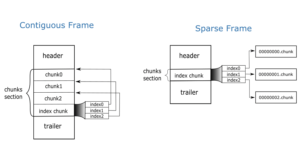
As for the data container, we are going to use the super-chunk object that comes with the Blosc2 library. A super-chunk is a data structure that is meant to host many data chunks in a compressed form, and that has some interesting features; more specifically:

• Compactness: everything in a super-chunk is designed to take as little space as possible, not only by using compression, but also my minimizing the amount of associated metadata (like indexes).

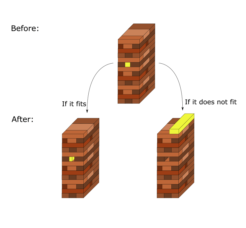
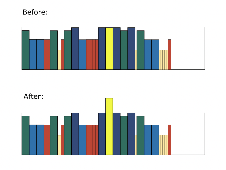
• Small fragmentation: by splitting the data in large enough chunks that are contiguous, the resulting structure ends stored in memory with a pretty small amount of 'holes' in it, allowing a more efficient memory management by both the hardware and the software.

• Support for contexts: useful when we have different threads and we want to decompress data simultaneously. Assigning a context per each thread is enough to allow the simultaneous use of the different cores without badly interfering with each other.

• Easy access to chunks: an integer is assigned to the different chunks so that requesting a specific chunk is just a matter of specifying its number and then it gets decompressed and returned in one shot. So pointer arithmetic is replaced by indexing operations, making the code less prone to get severe errors (e.g. if a chunk does not exist, an error code is returned instead of creating a segmentation fault).

If you are curious on how the super-chunk can be created and used, just check the sources for the benchmark used for this blog.

Regarding the computing algorithm, I will use one that follows the principles of the blocking computing technique: for every chunk, bring it to the CPU, decompress it (so that it stays in cache), run all the necessary operations on it, and then proceed to the next chunk:

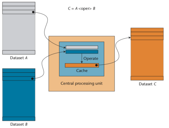
For implementation details, have a look at the benchmark sources.

Also, and in order to allow maximum efficiency when performing multi-threaded operations, the size of each chunk in the super-chunk should fit in non-shared caches (namely, L1 and L2 in modern CPUs). This optimization avoids concurrent access to bus caches as much as possible, thereby allowing dedicated access to data caches in each core.

For our experiments below, we are going to choose a chunksize of 4,000 elements because Blosc2 needs 2 internal buffers for performing the decompression besides the source and destination buffer. Also, we are using 32-bit (4 bytes) float values for our exercise, so the final size used in caches will be 4,000 * (2 + 2) * 4 = 64,000 bytes, which should fit comfortably in L2 caches in most modern CPU architectures (which normally sports 256 KB or even higher). Please note that finding an optimal value for this size might require some fine-tuning, not only for different architectures, but also for different datasets.

The Precipitation Dataset

There are plenty of datasets out there exposing different data distributions so, depending on your scenario, your mileage may vary. The dataset chosen here is the result of a regional reanalysis covering the European continent, and in particular, the precipitation data in a certain region of Europe. Computing the aggregation of this data is representative of a catchment average of precipitation over a drainage area.

Caveat: For the sake of easy reproducibility, for building the 100 million dataset I have chosen a small geographical area with a size of 150x150 and reused it repeatedly so as to fill the final dataset completely. As the size of the chunks is lesser than this area, and the super-chunk (as configured here) does not use data redundancies from other chunks, the results obtained here can be safely extrapolated to the actual dataset made from real data (bar some small differences).

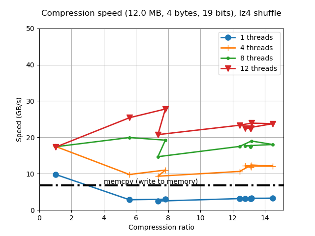
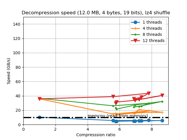
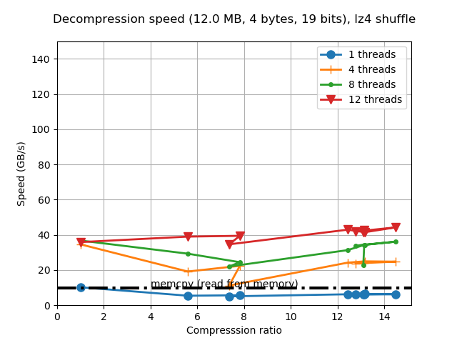
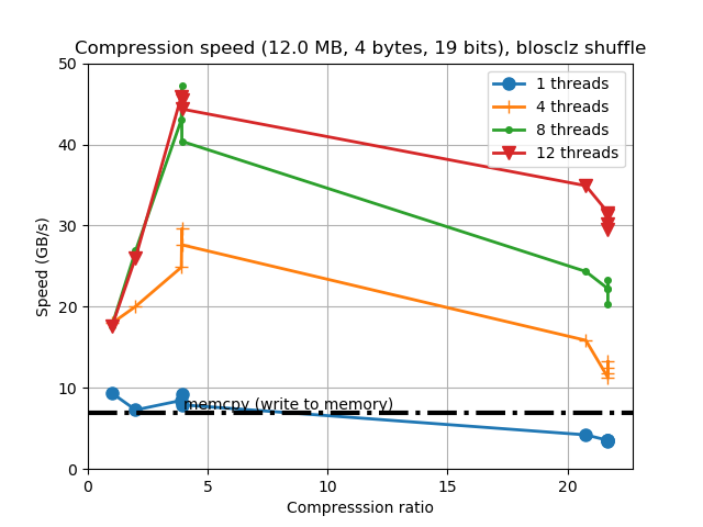
Choosing the Compression Codec

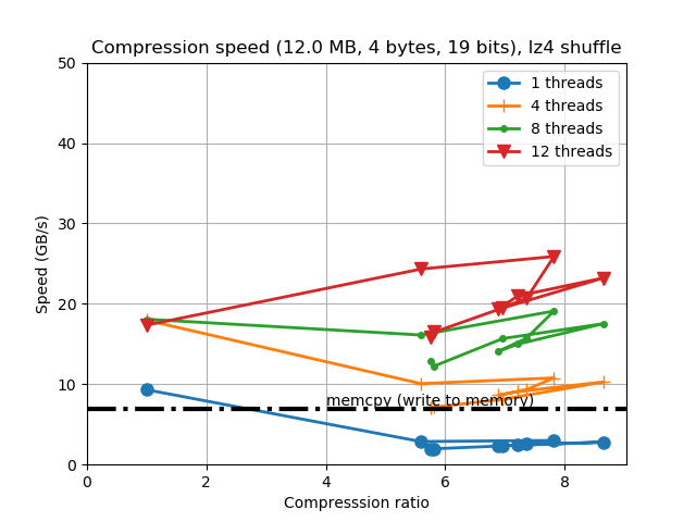
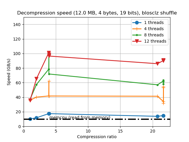
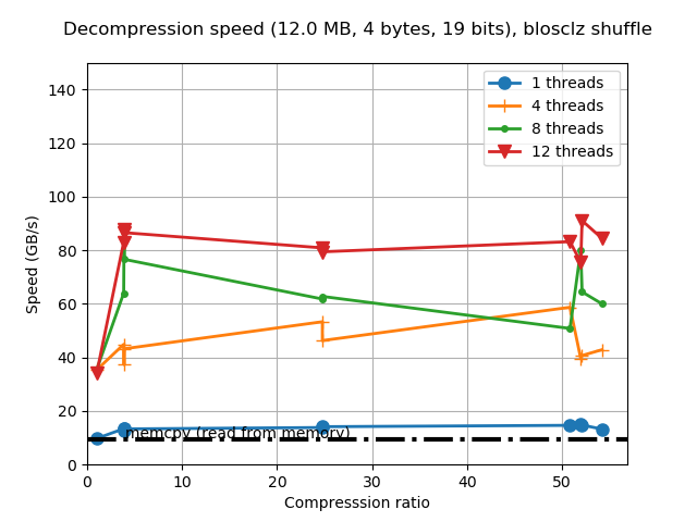
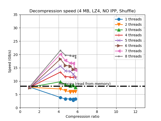
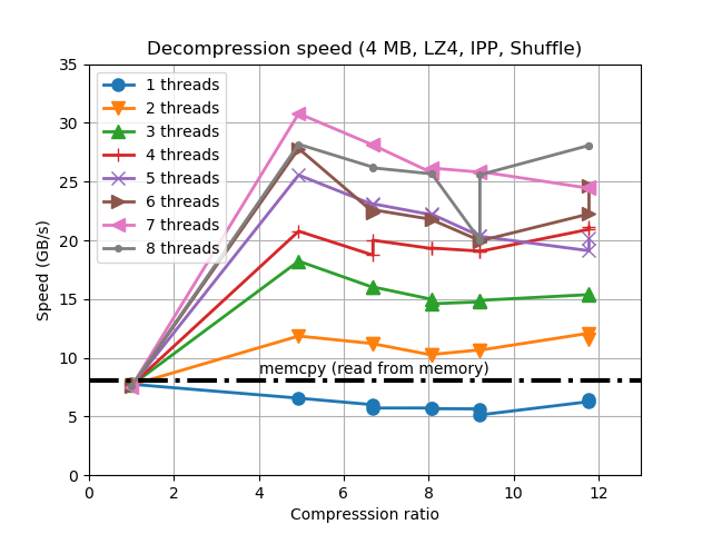
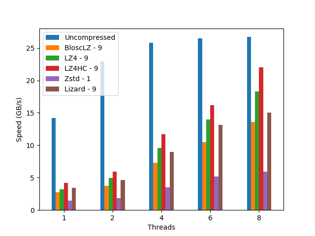
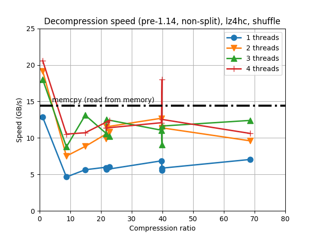
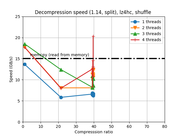
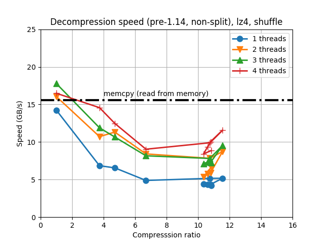
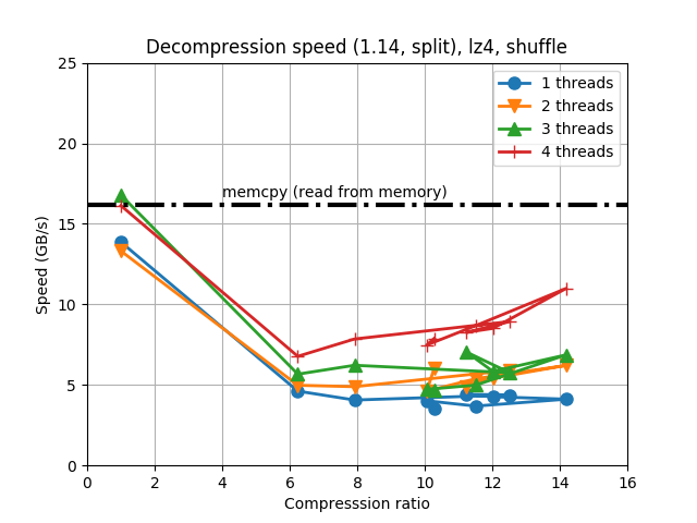
When determining the best codec to use inside Blosc2 (it has support for BloscLZ, LZ4, LZ4HC, Zstd, Zlib and Lizard), it turns out that they behave quite differently, both in terms of compression and speed, with the dataset they have to compress and with the CPU architecture in which they run. This is quite usual, and the reason why you should always try to find the best codec for your use case. Here we have how the different codecs behaves for our precipitation dataset in terms of decompression speed for our reference platform (Intel Xeon E3-1245):

In this case LZ4HC is the codec that decompress faster for any number of threads and hence, the one selected for the benchmarks for the reference platform. A similar procedure has been followed to select the codec for the CPUs. The selected codec for every CPU will be conveniently specified in the discussion of the results below.

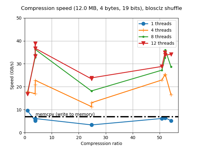
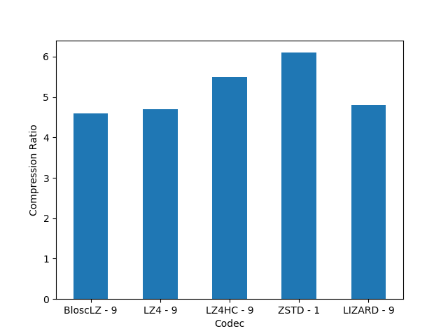
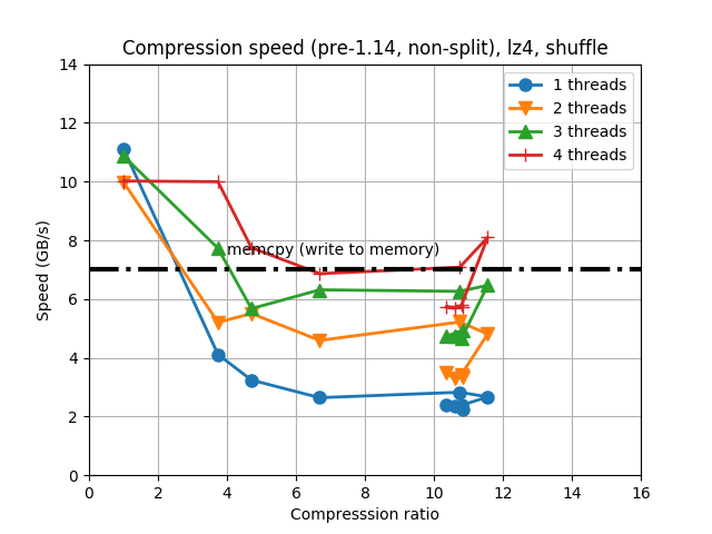
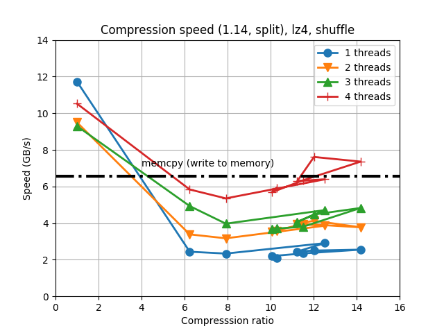
For completeness, I am also showing the compression ratios achieved by the different codecs for the precipitation dataset. Although there are significant differences for them, these usually come at the cost of compression/decompression time. At any rate, even though compression ratio is important, in this blog we are mainly interested in the best decompression speed, so we will use this latter as the only important parameter for codec selection.

Results on Different CPUs

Now it is time to see how our compressed sum algorithm performs compared with the original uncompressed one. However, as not all the CPUs are created equal, we are going to see how different CPUs perform doing exactly the same computation.

Reference CPU: Intel Xeon E3-1245 v5 4-Core processor @ 3.50GHz

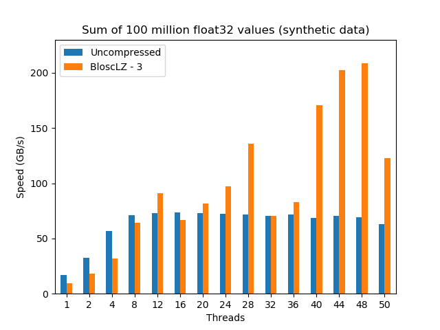
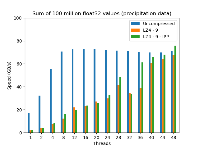
This is a mainstream, somewhat 'small' processor for servers that has an excellent price/performance ratio. Its main virtue is that, due to its small core count, the CPU can be run at considerably high clock speeds which, combined with a high IPC (Instructions Per Clock) count, delivers considerable computational power. These results are a good baseline reference point for comparing other CPUs packing a larger number of cores (and hence, lower clock speeds). Here it is how it performs:

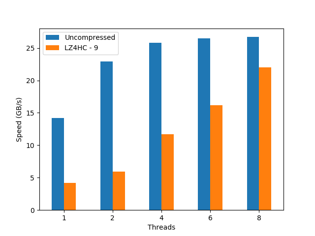
We see here that, even though the uncompressed dataset does not scale too well, the compressed dataset shows a nice scalability even when using using hyperthreading (> 4 threads); this is a remarkable fact for a feature (hyperthreading) that, despite marketing promises, does not always deliver 2x the performance of the physical cores. With that, the performance peak for the compressed precipitation dataset (22 GB/s, using LZ4HC) is really close to the uncompressed one (27 GB/s); quite an achievement for a CPU with just 4 physical cores.

AMD EPYC 7401P 24-Core Processor @ 2.0GHz

This CPU implements EPYC, one of the most powerful architectures ever created by AMD. It packs 24 physical cores, although internally they are split into 2 blocks with 12 cores each. Here is how it behaves:

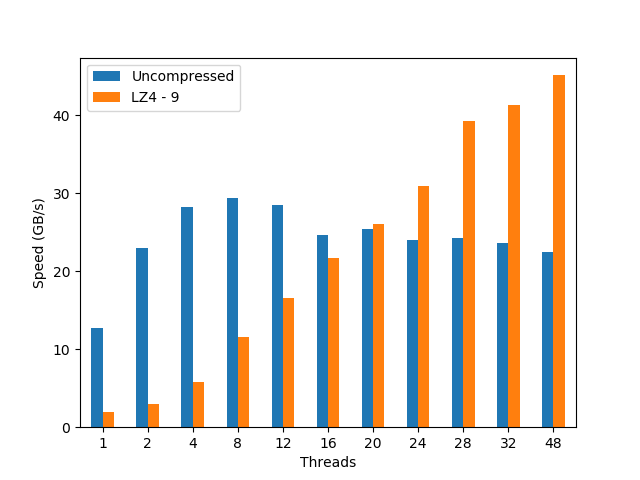
Stalling at 4/8 threads, the EPYC scalability for the uncompressed dataset is definitely not good. On its hand, the compressed dataset behaves quite differently: it shows a nice scalability through the whole range of cores in the CPU (again, even when using hyperthreading), achieving the best performance (45 GB/s, using LZ4) at precisely 48 threads, well above the maximum performance reached by the uncompressed dataset (30 GB/s).

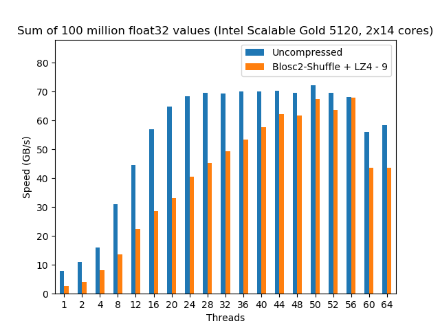
Intel Scalable Gold 5120 2x 14-Core Processor @ 2.2GHz

Here we have one of the latest and most powerful CPU architectures developed by Intel. We are testing it here within a machine with 2 CPUs, each containing 14 cores. Here’s it how it performed:

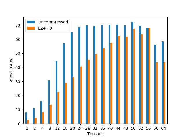
In this case, and stalling at 24/28 threads, the Intel Scalable shows a quite remarkable scalability for the uncompressed dataset (apparently, Intel has finally chosen a good name for an architecture; well done guys!). More importantly, it also reveals an even nicer scalability on the compressed dataset, all the way up to 56 threads (which is expected provided the 2x 14-core CPUs with hyperthreading); this is a remarkable feat for such a memory bandwidth beast. In absolute terms, the compressed dataset achieves a performance (68 GB/s, using LZ4) that is very close to the uncompressed one (72 GB/s).

Cavium ARMv8 2x 48-Core

We are used to seeing ARM architectures powering most of our phones and tablets, but seeing them performing computational duties is far more uncommon. This does not mean that there are not ARM implementations that cannot power big servers. Cavium, with its 48-core in a single CPU, is an example of a server-grade chip. In this case we are looking at a machine with two of these CPUs:

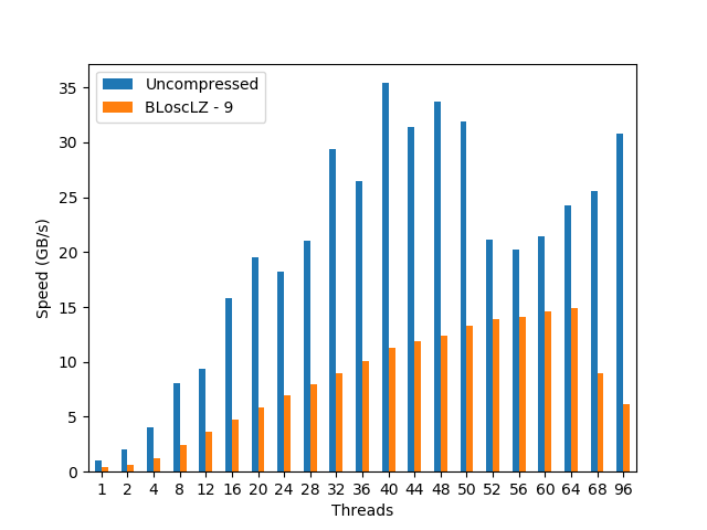
Again, we see a nice scalability (while a bit bumpy) for the uncompressed dataset, reaching its maximum (35 GB/s) at 40 threads. Regarding the compressed dataset, it scales much more smoothly, and we see how the performance peaks at 64 threads (15 GB/s, using BloscLZ) and then drops significantly after that point (even if the CPU still has enough cores to continue the scaling; I am not sure why is that). Incidentally, the BloscLZ codec being the best performer here is not a coincidence as it recently received a lot of fine-tuning for ARM.

What We Learned

We have explored how to use compression in an nearly optimal way to perform a very simple task: compute an aggregation out of a large dataset. With a basic understanding of the cache and memory subsystem, and by using appropriate compressed data structures (the super-chunk), we have seen how we can easily produce code that enables modern CPUs to perform operations on compressed data at a speed that approaches the speed of the same operations on uncompressed data (and sometimes exceeding it). More in particular:

1. Performance for the compressed dataset scales very well on the number of threads for all the CPUs (even hyperthreading seems very beneficial at that, which is a welcome surprise).

2. The CPUs that benefit the most from compression are those with relatively low memory bandwidth and CPUs with many cores. In particular, the EPYC architecture is a good example and we have shown how the compressed dataset can operate 50% faster that the uncompressed one.

3. Even when using CPUs with a low number of cores (e.g. our reference CPU, with only 4) we can achieve computational speeds on compressed data that can be on par with traditional, uncompressed computations, while saving precious amounts of memory and disk space.

4. The appropriate codec (and other parameters) to use within Blosc2 for maximum performance can vary depending on the dataset and the CPU used. Having a way to automatically discover the optimal compression parameters would be a nice addition to the Blosc2 library.

Final Thoughts

To conclude, it is interesting to remember here what Linus Torvalds said back in 2006 (talking about the git system that he created the year before):

[...] git actually has a simple design, with stable and reasonably well-documented data structures. In fact, I'm a huge proponent of designing your code around the data, rather than the other way around, and I think it's one of the reasons git has been fairly successful. [...] I will, in fact, claim that the difference between a bad programmer and a good one is whether he considers his code or his data structures more important. Bad programmers worry about the code. Good programmers worry about data structures and their relationships.

Of course, we all know how drastic Linus can be in his statements, but I cannot agree more on how important is to adopt a data-driven view when designing our applications. But I'd go further and say that, when trying to squeeze the last drop of performance out of modern CPUs, data containers need to be structured in a way that leverages the characteristics of the underlying CPU, as well as to facilitate the application of the blocking technique (and thereby allowing compression to run efficiently). Hopefully, installments like this can help us explore new possibilities to break down the memory wall that bedevils modern computing.

Acknowledgements

Thanks to my friend Scott Prater for his great advices on improving my writing style, Dirk Schwanenberg for pointing out to the precipitation dataset and for providing the script for reading it, and Robert McLeod, J. David Ibáñez and Javier Sancho for suggesting general improvements (even though some of their suggestions required such a big amount of work that made me ponder about their actual friendship :).

Appendix: Software used

For reference, here it is the software that has been used for this blog entry:

• OS: Ubuntu 18.04

• Compiler: GCC 7.3.0

• C-Blosc2: 2.0.0a6.dev (2018-05-18)

The #215 issue

Recently, a C-Blosc user filed an issue describing how buffers created with a modern version of C-Blosc (starting from 1.11.0) were not able to be decompressed with an older version of the library (1.7.0), i.e. C-Blosc was effectively breaking the so-called forward-compatibility. After some investigation, it turned out that the culprit was an optimization that was introduced in 1.11.0 in order to allow better compression ratios and in some cases, better speed too.

Not all the codecs inside C-Blosc were equally affected; the ones that are experiencing the issue are LZ4, LZ4HC and Zlib (quite luckily, BloscLZ, the default codec, is not bitten by this and should be forward compatible probably til 1.0.0); that is, when a user is using a modern C-Blosc library (> 1.11.0) and is using any of the affected codecs, there are situations (namely when the shuffle or bitshuffle filter are active and the buffers to be compressed are larger than 32 KB) that the result cannot be decompressed with older versions (< 1.11.0).

Why this occurred?

Prior to 1.11.0, Blosc has traditionally split the internal blocks (the different pieces in which the buffer to be compressed is divided) into smaller pieces composed by the same significant bytes that the shuffle filter has put together. The rational for doing this is that these pieces are, in many cases, hosting values that are either zeros or very close byte values (this is why shuffle works well in general for binary data), and asking the codec to compress these split-blocks separately was quite less effort than compressing a complete block hence providing more speed).

However, I realized that the so-called High Compression Ration codecs (the HCR codecs inside BLosc are LZ4HC, Zlib and Zstd) generally benefited from this split not happening (the reason is clear: more data means more opportunities for finding more duplicates) and in some cases, the speed was better too. So, in C-Blosc 1.11.0, I decided that the split was not going to happen by default for HCR codecs (in the last minute I decided to include LZ4 too, for which the experiments showed a noticeable performance bump too, see below). Fortunately, the Zstd codec was introduced (in an out-of-beta way) at the very same 1.11.0 release than this split-block change, so in practice data compressed with the Zstd codec is not affected by this.

New forward compatibility enforcement policy

Although this change was deliberate and every measure was put in making it backward compatible (i.e. new library versions could read buffers compressed with older versions), I was not really aware of the inconveniences that the change was putting for people creating data files using newer versions of the library and expecting these to be read with older versions.

So in order to prevent something like this to happen again, I decided that forward compatibility is going to be enforced for future releases of C-Blosc (just for 1.x series; C-Blosc 2.x should be just backward compatible with 1.x). By the way, this new forward compatibility policy will require a significantly more costly release procedure, as different libraries for a specific set of versions have to be manually re-created; if you know a more automatic way to test forward compatibility with old versions of a library, I'd love to hear your comments.

Measures taken and new split mode

In order to alleviate this forward incompatibility issue, I decided to revert the split change introduced in 1.11.0 in forthcoming 1.14.0 release. That means that, by default, compressed buffers created with C-Blosc 1.14.0 and on will be forward compatible with all the previous C-Blosc libraries (till 1.3.0, which was when support for different codecs was introduced). That is, the only buffers that will pose problems to be decompressed with old versions are those created with a C-Blosc library with versions between 1.11.0 and 1.14.0 and using the shuffle/bitshuffle filter in combination with the LZ4, LZ4HC or Zlib codecs.

For fine-tuning how the block-split would happen or not, I have introduced a new API function, void blosc_set_splitmode(int mode), that allows to select the split mode that is going to be used during the compression. The split modes that can take the new function are:

• BLOSC_FORWARD_COMPAT_SPLIT

• BLOSC_AUTO_SPLIT

• BLOSC_NEVER_SPLIT

• BLOSC_ALWAYS_SPLIT

BLOSC_FORWARD_COMPAT_SPLIT offers reasonably forward compatibility (i.e. Zstd still will not split, but this is safe because it was introduced at the same time than the split change in 1.11.0), BLOSC_AUTO_SPLIT is for nearly optimal results (based on heuristics; this is the same approach than the one introduced in 1.11.0), BLOSC_NEVER_SPLIT and BLOSC_ALWAYS_SPLIT are for the user interested in experimenting for getting best compression ratios and/or speed. If blosc_set_splitmode() is not called, the default mode will be BLOSC_FORWARD_COMPAT_SPLIT.

Also, the user will be able to specify the split mode by using the BLOSC_SPLITMODE variable environment. If that variable exists in the environment, and has any value among:

• 'BLOSC_FORWARD_COMPAT_SPLIT'

• 'BLOSC_AUTO_SPLIT'

• 'BLOSC_NEVER_SPLIT'

• 'BLOSC_ALWAYS_SPLIT'

this will select the corresponding split mode.

How this change affects performance

So as to allow to visualize at a glance the differences in performance that the new release is introducing, let's have a look at the impact on two of the most used codecs inside C-Blosc: LZ4 and LZ4HC. In the plots below the left side is the pre-1.14.0 version (non-split blocks) and on the right, the forthcoming 1.14.0 (split blocks). Note that I am using here the typical synthetic benchmarks for C-Blosc, so expect a different outcome for your own data.

Let's start by LZ4HC, a High Compression Ratio codec (and the one that triggered the initial report of the forward compatibility issue). When compressing, we have this change in behavior:

For LZ4HC decompression:

For LZ4HC one can see that, when using non-split blocks, it can achieve better compression ratios (this is expected, as the block sizes are larger). Speed-wise the performance is quite similar, with maybe some advantage for split blocks (expected as well). As the raison d'être for HCR codecs is maximize the compression ration, that was the reason why I did the split change for LZ4HC in 1.11.0.

And now for LZ4, a codec meant for speed (although it normally gives pretty decent results in compression ratio). When compressing, here it is the change:

For LZ4 decompression:

So, here one can see that when using Blosc pre-1.14 (i.e. non-split blocks) we are getting a bit less compression ratio than for the forthcoming 1.14, which even if counter-intutive, it matches my experience with non-HCR codecs. Speed-wise the difference is not that much during compression; however, decompression is significantly faster with non-split blocks. As LZ4 is meant for speed, this was possibly the reason that pushed me towards making non-split blocks by default for LZ4 in addition to HCR codecs in 1.11.0.

Feedback

If you have suggestions on this forward compatibility issue or the solution that has been implemented, please shout!

Appendix: Hardware and software used

For reference, here it is the configuration that I used for producing the plots in this blog entry.

• CPU: Intel Xeon E3-1245 v5 @ 3.50GHz (4 physical cores with hyper-threading)

• OS: Ubuntu 16.04

• Compiler: GCC 6.3.0

• C-Blosc: 1.13.7 and 1.14.0 (release candidate)

• LZ4: 1.8.1