Optimization tips
This page collects small idioms that make a measurable difference in speed or memory (often both). Each one is backed by a small benchmark in bench/optim_tips/, which you can run yourself — see the bench/optim_tips README.
Numbers below were measured on an Apple M4 Pro Mac Mini (macOS, Python 3.14); absolute values will differ on your machine, but the direction and rough magnitude of each effect should not.
Build large arrays with blosc2’s own constructors
Constructors like blosc2.arange(), blosc2.linspace() and blosc2.fromiter() fill an NDArray chunk by chunk, using multiple threads. Building the same array in NumPy first and compressing it with asarray() means holding the whole thing uncompressed in memory at once.
# Avoid: materializes the full array in NumPy first
a = blosc2.asarray(np.linspace(0, 1, N))

# Prefer: fills the NDArray chunk by chunk
a = blosc2.linspace(0, 1, N)
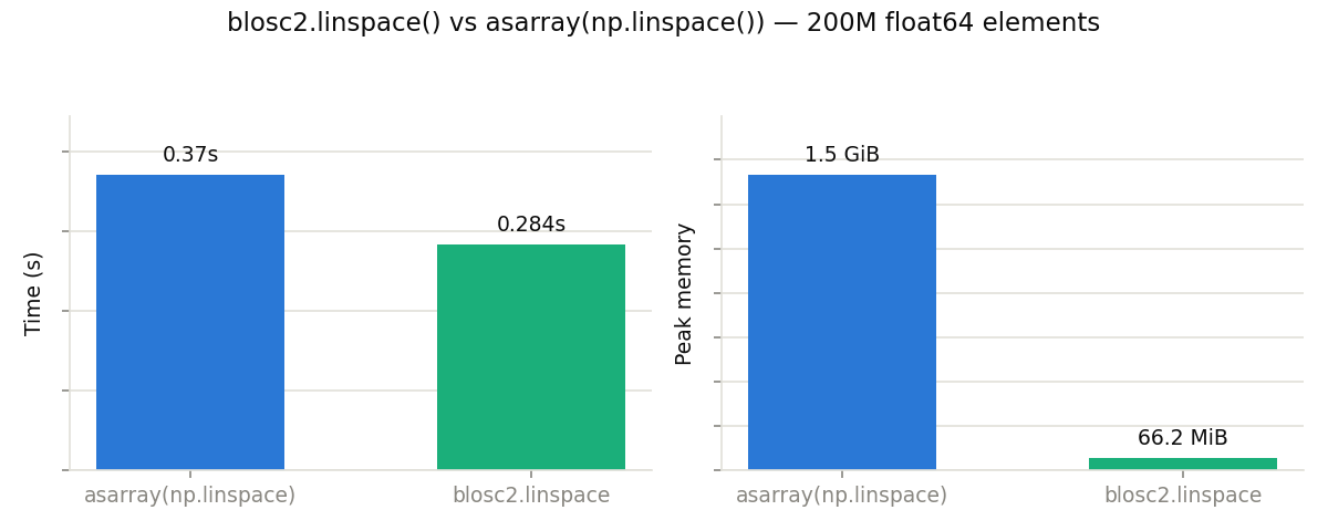
At 200M float64 elements, the constructor was ~1.5x faster and used ~16x less peak memory, and the memory gap widens with array size — the naive path’s memory is O(N), while the constructor’s stays roughly O(chunk size) for compressible enough data. The same applies to arange() and fromiter().
Benchmark for this tip: tip_01_constructors.py
Broadcast small operands into large, on-disk arrays
The same idea extends past the constructors: when a large array is a combination of smaller ones, build it as a lazy expression over broadcast blosc2 operands and compute() it directly to a file. Blosc2 broadcasts chunk by chunk, so the full uncompressed result never exists anywhere — only the small operands and one chunk at a time. NumPy broadcasting, by contrast, materializes the whole thing before asarray() gets a chance to compress it.
# Avoid: an 800 MiB NumPy array exists before a single byte is compressed
cols = np.arange(COLS, dtype=np.float64)
rows = np.arange(0, N * 0.001, 0.001, dtype=np.float64).reshape(N, 1)
a = blosc2.asarray(rows + cols, chunks=(CHUNK, COLS), urlpath="big.b2nd", mode="w")

# Prefer: two small operands, broadcast and evaluated chunk by chunk to disk
cols = blosc2.arange(COLS, dtype=np.float64)
rows = blosc2.arange(0, N * 0.001, 0.001, dtype=np.float64, shape=(N, 1))
a = (rows + cols).compute(chunks=(CHUNK, COLS), urlpath="big.b2nd", mode="w")
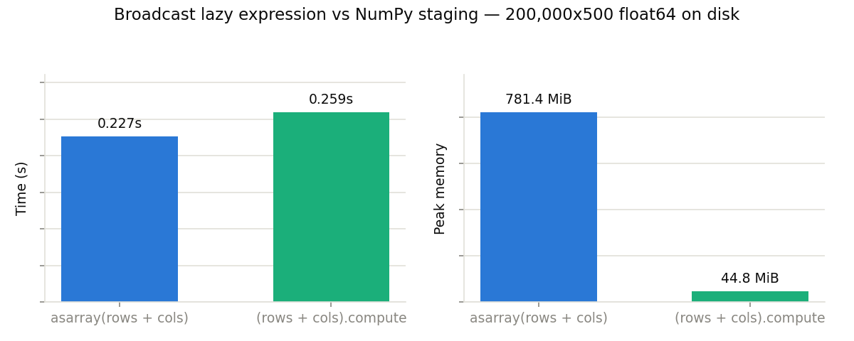
Both produce bit-identical files. For a 200,000x500 float64 array (~800 MiB uncompressed), the broadcast expression used ~26x less peak memory — the peak is a handful of chunks, not the whole array — at essentially the same speed. Memory is the point here: the naive path is O(N) and stops working when the array outgrows RAM, while the broadcast path doesn’t care how big the result is.
This works for any expression over operands blosc2 can broadcast, not just two arange()s: an existing on-disk NDArray times a per-column scale vector, a 2D field plus a 1D offset, and so on. The shape rules are NumPy’s; the lazy expressions tutorial has a worked example.
Benchmark for this tip: tip_12_broadcast_build.py
Generate arrays with DSL kernels
The constructors from the previous tip are not magic: internally, blosc2.arange() is a one-line DSL kernel (start + _flat_idx * step) that blosc2 compiles to native code and evaluates chunk by chunk, using multiple threads. The same machinery — a blosc2.dsl_kernel-decorated function handed to blosc2.lazyudf() — is open to you, for any array whose value is a function of its index.
As a worked example, let’s build a random constructor from scratch: hash the element index (here with a classic integer hash), and every chunk can be filled independently, in parallel, reproducibly for a given seed. Blosc2 ships a proper one these days — see Random Functions — but writing a small version by hand is the clearest way to see what the machinery does.
@blosc2.dsl_kernel
def random_int32(seed):
    x = _flat_idx ^ seed
    x = (((x >> 16) ^ x) * 0x45D9F3B) & 0xFFFFFFFF
    x = (((x >> 16) ^ x) * 0x45D9F3B) & 0xFFFFFFFF
    return (x >> 16) ^ x  # full [-2^31, 2^31) range


# Avoid: materializes the full array with NumPy first
rng = np.random.default_rng(42)
a = blosc2.asarray(
    rng.integers(-(2**31), 2**31, size=N, dtype=np.int32), cparams={"clevel": 0}
)

# Prefer: the kernel fills the NDArray chunk by chunk, in parallel
lazy = blosc2.lazyudf(random_int32, (42,), dtype=np.int32, shape=(N,))
a = lazy.compute(cparams={"clevel": 0})
(clevel=0 because random data is incompressible — don’t pay the codec for nothing.)
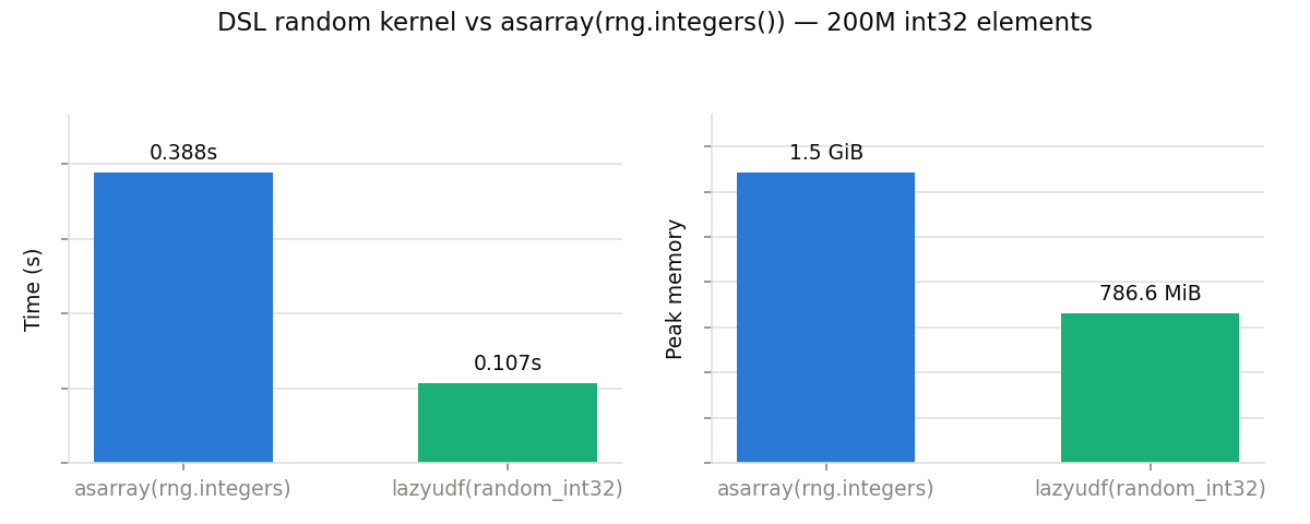
At 200M int32 elements, the DSL kernel was ~3.6x faster and used ~1.9x less peak memory than generating with NumPy and compressing via asarray() — the peak is just the result itself, since the full NumPy staging array never exists.
The output passes light uniformity checks against NumPy’s PCG64 (the benchmark script prints them) — good enough for synthetic data, benchmarks and test fixtures, but this hand-rolled hash is not a substitute for a real generator. For statistically rigorous work such as Monte Carlo, use blosc2.random, which gives you NumPy-quality streams (one independent SeedSequence per chunk) and keeps the chunk-parallel generation. The benchmark source explains the hash design and the DSL integer-arithmetic rules it relies on; see also the DSL syntax reference.
Benchmark for this tip: tip_11_dsl_random.py
Understanding @blosc2.jit compile control flow
There are two routes the @blosc2.jit decorator can take because they are good at different things:
No control flow → tracing (the default).
jitcalls your function once with proxy operands, records theLazyExprit builds, and evaluates that expression vectorized over whole chunks. This is the faster route for plain elementwise math.Control flow → the whole function is compiled. A traced call only ever walks one path through an
ifor a loop, so the other paths would be silently lost. So whenjitsees control flow and the body fits the DSL grammar, it compiles the entire function with the same miniexpr engine that enables the@blosc2.dsl_kerneldecorator and runs the compiled kernel chunk by chunk.
In short: you can write if, for and while inside a @blosc2.jit-decorated function and they will work as intended, provided the body sticks to the DSL grammar.
An example: Mandelbrot escape times
Escape-time counting is a per-pixel loop with an early break — exactly the scenario that tracing/vectorizing cannot represent.
Let’s compute the escape count of a 512×512 patch of the Mandelbrot set (max_iter=64) and compare the ways of running it:
def mandel_py(cr, ci, max_iter):  # plain Python: one loop per pixel
    zr = zi = 0.0
    n = 0
    while zr * zr + zi * zi <= 4.0 and n < max_iter:
        zr, zi = zr * zr - zi * zi + cr, 2 * zr * zi + ci
        n += 1
    return n


@blosc2.jit  # the same loop, written the natural way — jit detects the
# ^^^^^^^^^   # control flow at decoration time and compiles this kernel whole
def mandel_jit(cr, ci, max_iter):
    zr = 0.0
    zi = 0.0
    n = 0
    for _ in range(max_iter):
        if zr * zr + zi * zi > 4.0:
            break
        zr2 = zr * zr - zi * zi + cr
        zi = 2 * zr * zi + ci
        zr = zr2
        n += 1
    return n


iterations = mandel_jit(CR, CI, 64)  # CR, CI: the two float32 grids
The benchmark times four variants — the Python loop above, a vectorized NumPy mask iteration, the @blosc2.jit above, and the same kernel with @blosc2.jit(jit_backend="cc") (the system C compiler instead of the bundled tcc, with tradeoffs of its own below) — and checks that all of them return escape counts bit-identical to the pure-Python reference:
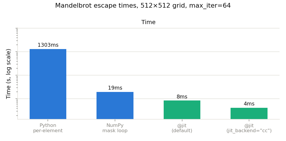
The default @blosc2.jit is ~160x faster than the Python loop and ~2.3x faster than the best plain-NumPy version (with jit_backend="cc", ~320x and ~4.7x).
Operands may equally be on-disk NDArray objects: the same kernel over blosc2.asarray() views of the two grids runs at the same speed and returns a plain NumPy array.
Gotcha: silent fallback to tracing
The DSL grammar is narrower than Python, and a body that misses it falls back to tracing silently — you only find out when the call fails. For example, the tuple assignment zr, zi = ... of the Python reference is not valid DSL program; that is why the jit version uses a zr2 temporary.
The DSL syntax reference has the full grammar. To turn that silent fallback into a hard error, decorate with @blosc2.jit(strict=True): it forces the DSL route and raises DSLSyntaxError at decoration time if the function cannot be compiled.
The opposite knob, strict=False, forces tracing even when there is control flow. On this function it fails loudly — tracing evaluates if zr * zr + zi * zi > 4.0 on an array, which raises ValueError. The dangerous case is a branch on a plain Python value instead (say if max_iter > 100): tracing records only the path that one call happened to take, and that path is then reused for every element, quietly. So use strict=False only when the branches depend on Python values, never on the arrays.
Element-wise functions still trace by default
If compiling the whole function is this good, why doesn’t jit do it for everything? Because without control flow, tracing usually wins: the traced expression is evaluated as one vectorized miniexpr over whole chunks, while a compiled kernel has to loop element by element.
Here is a heavy elementwise mix of transcendental functions:
@blosc2.jit  # using jit(strict=True) forces the DSL route
def heavy(x):
    return (
        np.sin(x)
        + np.cos(x * 2)
        + np.exp(x * 0.5) * np.sin(x * 3)
        + np.sqrt(np.abs(x))
        + np.log1p(np.abs(x))
    )
Measured over 8M float32 values:
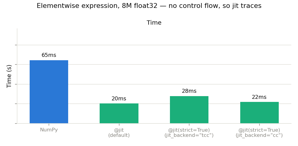
The first bar is the same expression in plain NumPy, as a scale anchor: all three jit routes beat it — the traced default by ~3.2x, and even the slowest of them, the forced DSL kernel on tcc, by ~2.3x.
Among the three, the default @blosc2.jit (which traces) is the faster route here: forcing the DSL route with strict=True is ~1.37x slower with the bundled tcc, and gets close to tracing when compiled with jit_backend="cc" (still ~1.07x slower; the plot shows the exact times). Note that jit_backend="cc" alone does not switch an elementwise function to the compiled route; it keeps tracing, at the same speed.
So, use strict=True when you want the compiled-kernel guarantee; but be aware that usually it may cost you speed.
Pros and cons of forcing the system compiler
jit_backend="cc" is faster in steady state on both kernels above — ~2.05x on the mandelbrot kernel and ~1.28x on the elementwise one — with identical results.
The price is the one-time compile. The benchmark measures it as the first call minus the steady state of the calls that follow it, in a fresh process:
kernel |
tcc (the default) |
cc, cold cache |
cc, warm cache |
|---|---|---|---|
mandelbrot |
3.2 ms |
233 ms |
1.3 ms |
elementwise |
4.0 ms |
253 ms |
2.9 ms |
tcc compiles in memory, so every process pays those few milliseconds again. cc writes a shared object into $TMPDIR/miniexpr-jit, keyed by a fingerprint of the kernel, its dtypes and the toolchain: only the first process on a machine pays the compiler.
So cc pays off for kernels you call repeatedly in the same run (or across runs), or when run time is much larger than compile time. It also requires a C compiler and a writable cache directory.
The same switch is available globally through the BLOSC_ME_JIT=cc environment variable, which wins over the keyword argument.
Benchmark for this tip: tip_15_jit_control_flow.py
Align your reads with the double partition
blosc2 arrays are partitioned twice: the array is split into chunks (the unit of storage and compression), and each chunk is subdivided into blocks (the unit of decompression, sized to fit CPU caches). A read that lands exactly on a partition boundary decompresses only the chunk or block it needs, while the same-sized read shifted off-grid straddles (and decompresses) extra ones.
You don’t have to pick the partitions yourself: let blosc2 choose them, then read them back from arr.chunks and arr.blocks to place your slice boundaries.
At the chunk level
NDArray.slice() has a fast path when both boundaries land on chunk boundaries: whole chunks are copied as-is, compressed, with no decompression at all. Regular reads also benefit — an aligned chunk-sized read decompresses one chunk instead of two.
arr = blosc2.asarray(data)  # let blosc2 pick the partitions
ch = arr.chunks[0]  # e.g. 1000 for a 16000×2000 float64 array

# Avoid: a chunk-sized read straddling two chunks → decompresses both
arr[ch // 2 : ch // 2 + ch, :]

# Aligned read: on the chunk grid → decompresses exactly one chunk
arr[ch : 2 * ch, :]

# Even better: slice() on chunk boundaries → copies chunks as-is, no decompress
arr.slice((slice(ch, 2 * ch), slice(None)))
At the block level
The same alignment principle applies at the block level: a block-aligned read decompresses exactly the blocks it needs. With auto-chosen blocks this effect is small — blocks are tiny by design — but if you configure larger blocks (say, for better compression ratios), keeping reads on the block grid pays off.
The slice() fast path, however, does not apply here: it only works at chunk boundaries, so slice() of a block-sized region still decompresses and recompresses:
big = blosc2.asarray(data, chunks=(4000, 2000), blocks=(100, 2000))
bl = big.blocks[0]

# Avoid: a block-sized read straddling two blocks → decompresses both
big[bl // 2 : bl // 2 + bl, :]

# Aligned read: on the block grid → decompresses exactly one block
big[bl : 2 * bl, :]

# slice() at block granularity → still decompresses + recompresses the chunk
big.slice((slice(bl, 2 * bl), slice(None)))
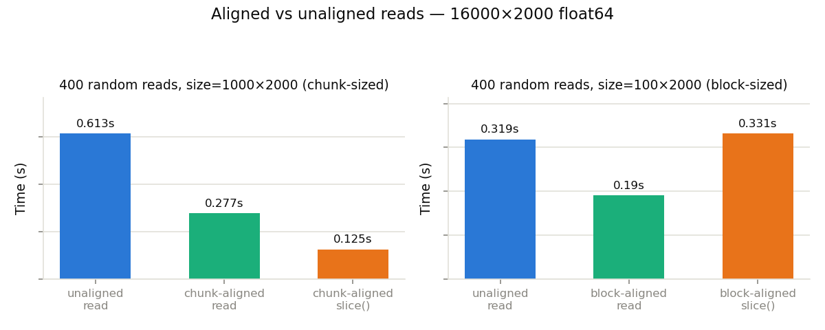
On a 16000×2000 float64 array, 400 chunk-sized reads aligned with the chunk grid were ~2.3× faster than the same reads shifted half a chunk off-grid, and a chunk-aligned slice() was ~11× faster again (no decompression), i.e. ~25× faster than the unaligned read. At the block level (with larger 1.6 MB blocks), 400 block-sized reads aligned with the block grid were ~2× faster. However, slice() at block granularity was no faster at all — slice() has to produce a valid compressed array with its own chunk layout, so it can only skip decompression when both boundaries land on chunk boundaries; at block granularity it still decompresses and recompresses.
Practically: reach for slice() when both boundaries land on chunk boundaries and you want a compressed result. Off that path it is strictly more work than arr[...] — and if you wanted NumPy at the end, you have paid to compress something you are about to throw away.
Benchmark for this tip: tip_02_chunk_aligned_slicing.py
Sorted top-k: stream from FULL indexes
A FULL index stores rows in sorted order. When all you need is the top (or
bottom) k rows, you can stream just that slice directly from the index
sidecar instead of materialising the full sorted permutation. Both
CTable and NDArray expose this.
CTable: sort_by(view=True)
CTable.sort_by(view=True) returns a
lightweight sorted view that gathers rows from the parent table on demand.
On a FULL-indexed column it streams straight from the index — the table is
never actually sorted at all:
t.create_index("temperature", kind=blosc2.IndexKind.FULL)

# Avoid: sorts (and copies) the whole table just to keep 10 rows
top10 = t.sort_by("temperature")[:10]

# Prefer: zero-copy view, streamed from the index
top10 = t.sort_by("temperature", view=True)[:10]
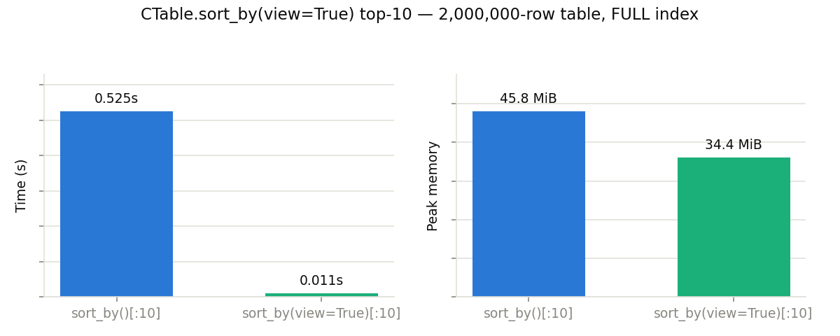
On a 20M-row table, the view form took ~99× less time and about 25% less
peak memory than a full sort_by(). The larger the table relative to
k, the bigger the gap, since the naive path’s cost is dominated by sorting
rows you’re about to discard.
Benchmark: tip_03_sort_by_view.py
NDArray: iter_sorted(start=-k)
For 1-D NDArray objects, NDArray.iter_sorted(start=-k) reads just the tail of the index sidecar,
avoiding the full permutation that argsort()
would materialise:
arr.create_index(kind=blosc2.IndexKind.FULL)

# Avoid: materialises all 20M positions just to keep 10
top10 = arr[arr.argsort()[-10:]]

# Prefer: reads only the last 10 entries from the sidecar
top10 = np.fromiter(arr.iter_sorted(start=-10), dtype=arr.dtype)
Descending and bottom-k work via step=-1:
list(arr.iter_sorted(start=-1, stop=-11, step=-1))  # top-10 descending
list(arr.iter_sorted(stop=10))  # bottom-10 ascending
list(arr.iter_sorted(start=9, stop=None, step=-1))  # bottom-10 descending
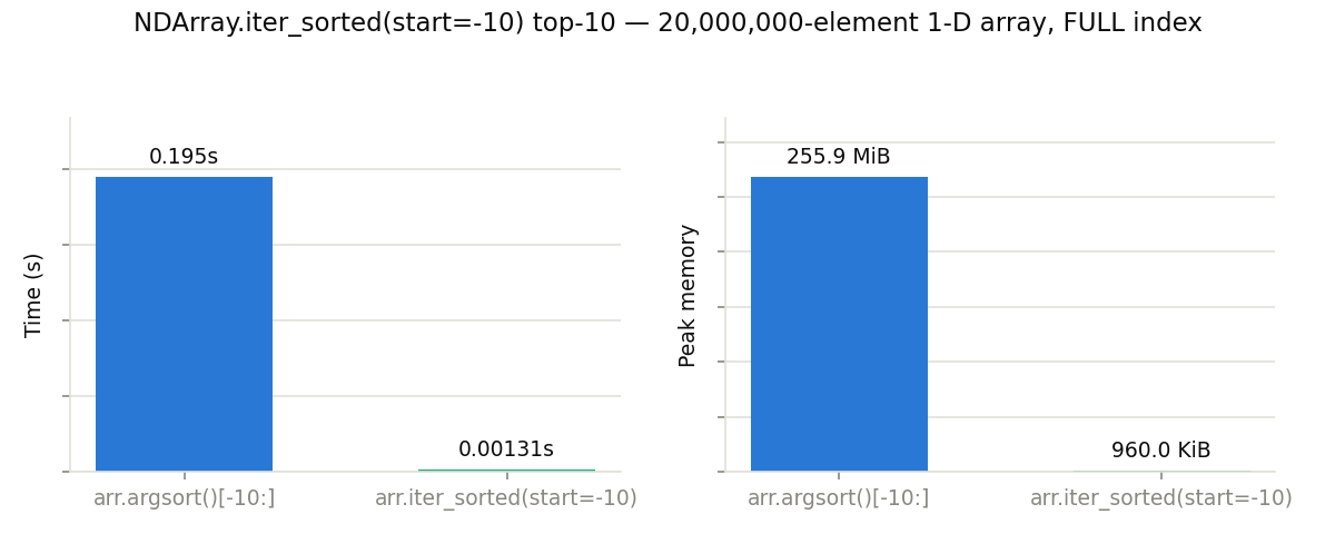
On a 20M-element float64 array, iter_sorted(start=-10) was ~149× faster
and used ~270× less peak memory than argsort()[-10:] — the latter
still materialises the full 20M-element positions array even when backed by a
FULL index.
Benchmark: tip_03b_ndarray_iter_sorted.py
Let SUMMARY indexes answer min()/max() directly
When closing a CTable, Blosc2 automatically builds SUMMARY indexes (per-block min/max) for its eligible scalar columns — this is on by default (create_summary_index=True). Column.min()/max() (and argmin()/argmax() inside group_by()) then answer from those precomputed summaries instead of decompressing the column at all.
# create_summary_index=True is the default; closing the table builds the index
with blosc2.CTable(Row, urlpath="t.b2d", mode="w") as t:
    t.extend(data)

t = blosc2.open("t.b2d")
hottest = t["temperature"].max()  # answered from the SUMMARY index
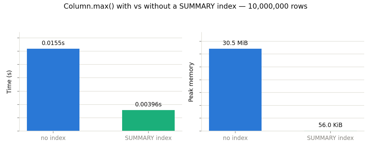
On a 10M-row column, the indexed max() took ~5x less time than without an index, and needed essentially no extra memory — it never touches the compressed column data at all.
The same SUMMARY indexes can also let a selective where() query skip whole blocks, but only when the column’s values are ordered or clustered enough that a block’s min/max range can exclude the predicate entirely. With independently random data every block spans nearly the full value range and there is nothing to skip — so the min()/max() speedup is the one you can always count on.
Benchmark for this tip: tip_04_summary_index_where.py
Reduce columns directly — don’t slice them first
t["col"][:] materializes the whole column as one big NumPy array. If all you want is a reduction, call it on the Column itself: sum(), mean(), min(), … work chunk by chunk and never hold the whole column decompressed at once — while still handling null values and deleted rows correctly.
# Avoid: decompresses the whole column into one NumPy array first
total = t["val"][:].sum()

# Prefer: chunk-wise reduction straight over the compressed column
total = t["val"].sum()
![col.sum() vs col[:].sum()](../_images/tip_05_column_reduce.png)
On a 250M-row column, col.sum() was ~1.6x faster, but more importantly it used ~62x less peak memory. For large tables the memory savings alone can be the deciding factor.
Benchmark for this tip: tip_05_column_reduce.py
Filtered reductions: push the predicate down with where=
The previous tip extends to filtered aggregates. The NumPy-style idiom — materialize the value column and the predicate column, build a boolean mask, then reduce — decompresses both columns in full just to keep a fraction of the rows. Column reductions accept a where= predicate instead, which is pushed down into the same chunk-wise scan: no intermediate arrays, no filtered view.
# Avoid: decompresses both full columns just to mask one of them
temp = t.temperature[:]
reg = t.region[:]
total = temp[reg == 3].sum()

# Prefer: the filter travels with the chunk-wise reduction
total = t.temperature.sum(where=t.region == 3)
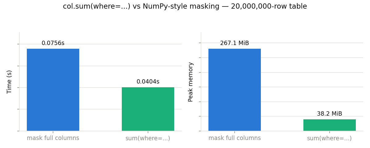
On a 20M-row table, the pushed-down form was ~2.2x faster and used ~7x less peak memory. Predicates can combine several columns too: t.amount.sum(where=(t.price < 300) & (t.qty > 0)).
Benchmark for this tip: tip_08_where_pushdown.py
Store unbounded text as utf8(), not fixed-width string()
A string column is fixed width because it uses NumPy’s <U dtype, which is UCS-4, so every row costs 4 × max_length bytes every time it is read — 800 bytes at max_length=200, whether the row holds three characters or two hundred. Compression hides the padding from the container, but not when materialized as a NumPy array. Now, you can use utf8() which stores UTF-8 natively and reads back as numpy.dtypes.StringDType, NumPy 2.0’s variable-width UTF-8 dtype; in this case rows cost what they weigh.
# Avoid, for text you can't bound: 800 bytes per row in memory on every read
title: str = blosc2.field(blosc2.string(max_length=200))

# Prefer: no declared width
title: str = blosc2.field(blosc2.utf8())
The measurements below use a 1 Mrow table of free text averaging 76 bytes per row (a few rows reach the 200-codepoint limit), in two versions: one where titles repeat a lot — 20k different ones spread over the million rows — and one where almost every row is different.
Reading full columns
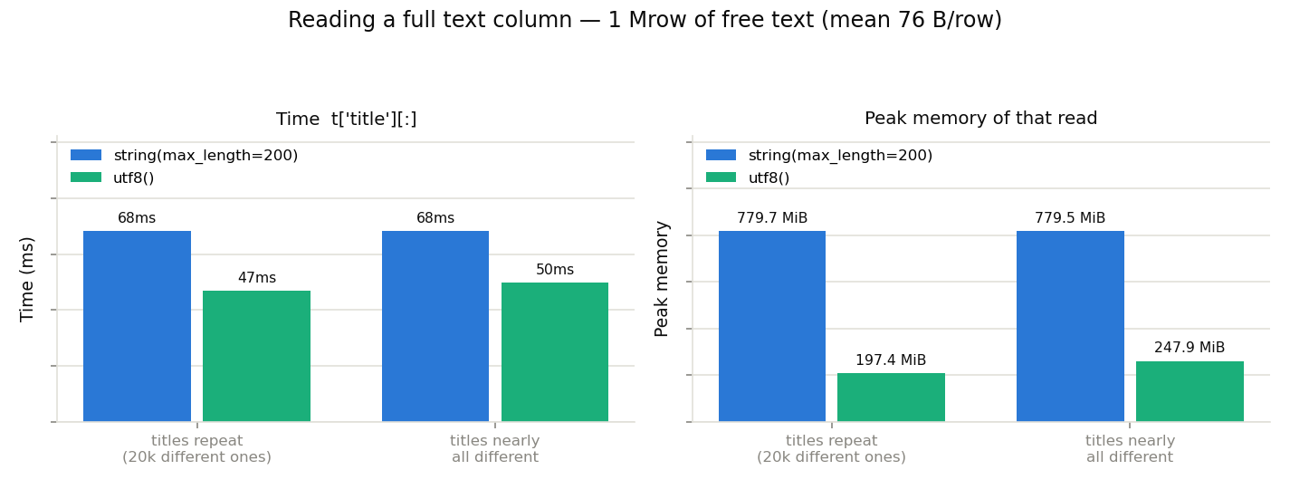
The time gap is real but modest — decompression dominates, and both flavours decompress about the same payload. The memory gap is the important one: the fixed-width array is rows × 800 B whatever the text actually weighs, so it does not depend on the data at all, while the utf8() array pays for the bytes that are there. How often titles repeat makes no difference either — the padding is charged per row, not per different value. And it scales linearly: the same column at 100 Mrows would need 80 GB of RAM to be read whole as string(200), against roughly a quarter of that as utf8().
Anything that materializes the column benefits from this — a NumPy comparison, to_pandas(), a plot. UTF-8 is also the ecosystem’s common currency: a utf8() column is int64 offsets plus a UTF-8 blob — Arrow’s large_string layout — so to_arrow() builds straight from the stored buffers, and pandas, Polars and DuckDB take it from there. Fixed width has to transcode UCS-4 on the way out. See utf8 and NumPy’s StringDType.
Querying columns, with and without a FULL index
Reading a column whole is one thing; finding values on it is another. where() never materializes the column — it scans chunk by chunk — so the memory blow-up above does not happen here at all. A FULL index replaces that scan with a direct lookup, on either flavour.
t.where("title == 'some exact title'")  # scans, one chunk at a time
t.create_index("title", kind=blosc2.IndexKind.FULL)
t.where("title == 'some exact title'")  # looks it up, no scan
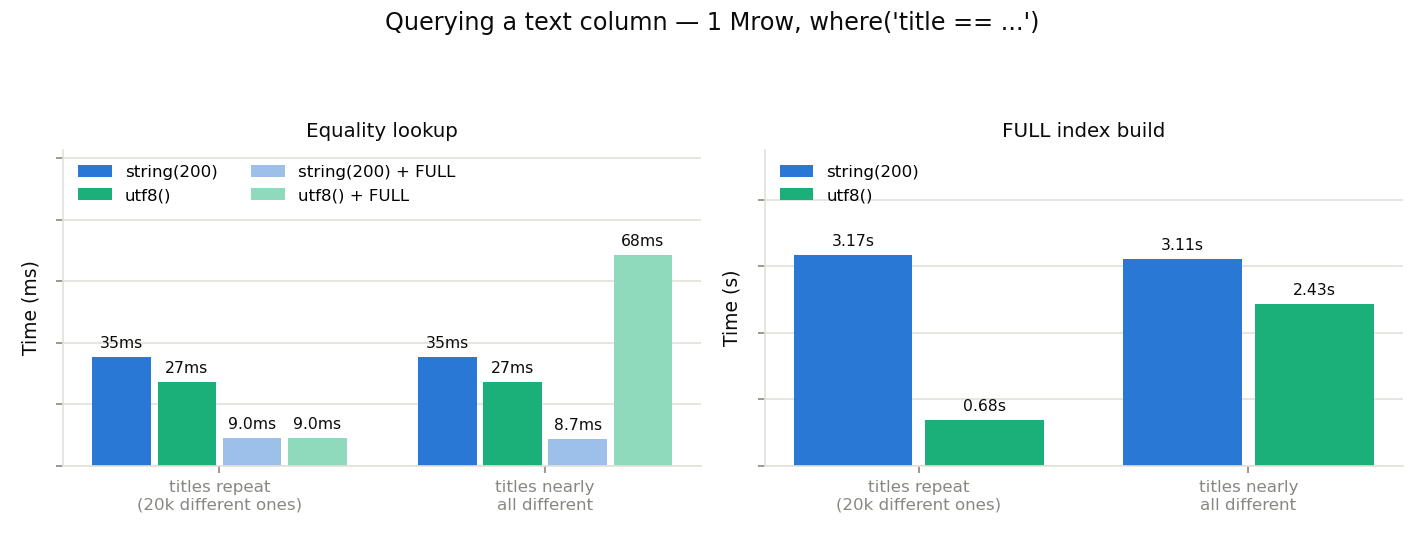
A utf8() column is indexed by alphabetical rank: the query literal is located by bisecting the index’s vocabulary, and the rows that match are a contiguous run of the sorted-positions sidecar. None of that depends on how many different values the column holds, so the index is worth having at either cardinality — a scan costs tens of milliseconds, a lookup a few. The first lookup of a session is the dearer one only because it opens the sidecars; later ones reuse them.
Changed in version 4.12.0: The literal is bisected out of the vocabulary sidecar. Earlier versions materialized the whole vocabulary on the first lookup, which on the near-unique column here cost ~62 ms and 739 MiB of peak memory instead of the new ~12 ms and 5.5 MiB.
string(200) answers just as directly, from the values themselves. utf8() is the faster of the two — comparing ranks is integer work — and by far the cheaper to build: ~4.6x faster when titles repeat, 1.3x when they do not, and 2.4 GiB of peak memory for the fixed-width build whatever the data, against 200 MiB / 1.2 GiB.
Caveat emptor: that sorted list is built once, so adding rows leaves it out of date: blosc2 falls back to a scan (correct results, no speedup) until you call rebuild_index(). Also, note how no index accelerates startswith or substring search, on any flavor.
Bytes on disk
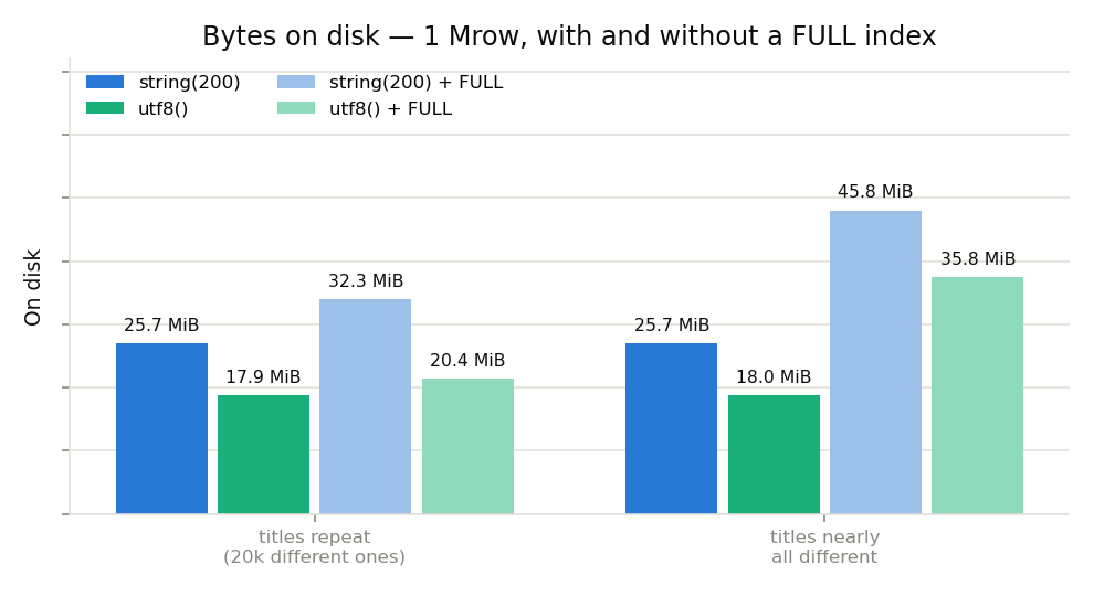
Compression squeezes most of the UCS-4 padding away, so the on-disk gap is nothing like the in-memory one — but it does not close: UCS-4 interleaves every real byte with zeros, and the codec still has to encode that, whether or not the text repeats. The FULL index is a sidecar file whose size follows the number of different values rather than the declared width — negligible when the text repeats, comparable to the column itself when it does not; utf8() is the cheaper of the two there as well.
The columns themselves barely differ between the two versions, which is worth knowing: compression works block by block, so repeated text only saves space when the repeats happen to sit close together, and here they are scattered at random. If your values repeat that heavily, dictionary() is the flavour built to exploit it — see the next tip.
Benchmark for this tip: tip_13_utf8_strings.py
Repeated text? Store it as dictionary()
The previous tip picks a flavour by length; this one corrects the choice by repetition. A dictionary() column stores one int32 code per row plus a single copy of each distinct value — Arrow’s dictionary encoding — so the text is written once and everything downstream works on integers.
# Fine for free text, but each row carries its own bytes
title: str = blosc2.field(blosc2.utf8())

# Prefer, when values repeat: one int32 code per row, one copy of each value
title: str = blosc2.field(blosc2.dictionary())
Same 1 Mrow column as the previous tip, now at three levels of repetition: 100 different titles, 20k different titles, and nearly all different.
Grouping
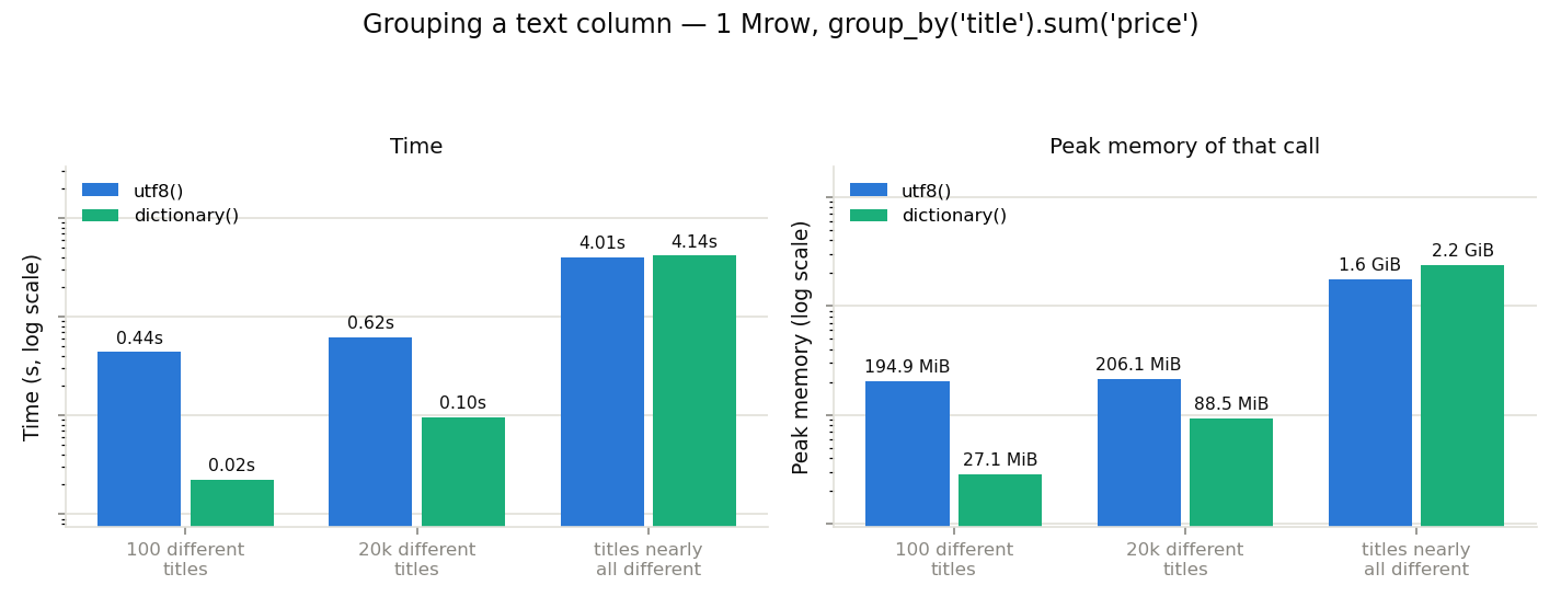
Grouping is what category columns are for, and it is where the layout pays off most: the codes are the group keys, so blosc2 tallies integers, while the utf8 column has to decode and hash every row’s text first. Note the log scale — at 100 different titles the gap is more than an order of magnitude, and it narrows as the number of groups grows. size() behaves just like sum() here; the shape of the aggregation is not what makes the difference.
Membership tests
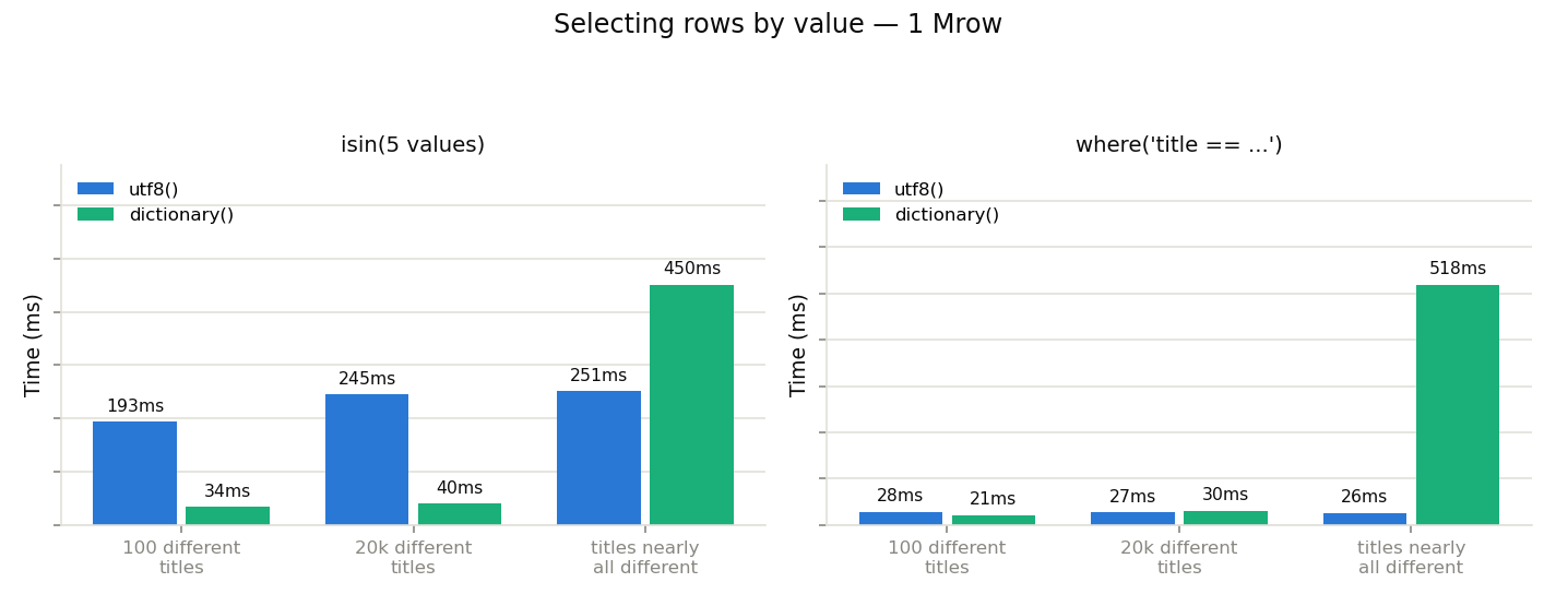
isin() is the clear win: the wanted values are translated to codes once, and the rest is an integer membership test, where utf8 must decode every row to compare it — which also explains the memory gap between them.
Plain == is a different story, and the figure says so: a single-value equality scan is already fast on a utf8 column, so there is nothing left for the codes to save. Switch flavour for grouping and isin(), not for ==.
Storing and reading
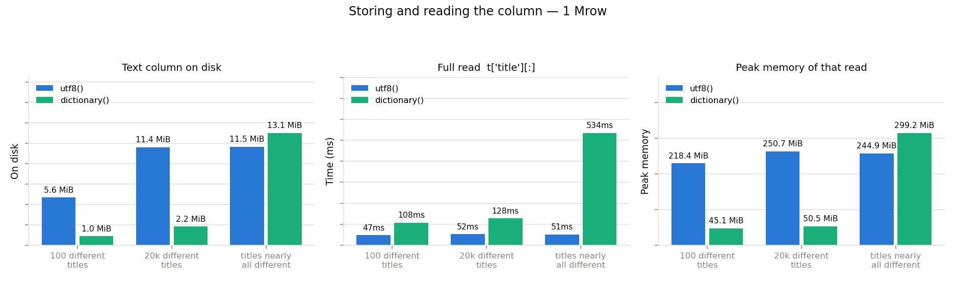
On disk, one int32 per row plus a single copy of each value beats storing every row’s bytes — and unlike compression, this does not depend on the repeats being clustered, which is exactly the limitation the previous tip ran into.
Reading the whole column back is the one place dictionary() is slower, since the codes have to become strings again. What you get is a Python list whose entries are shared str objects — one per distinct value, not one per row — which is why its peak memory is several times lower than utf8’s. It is also not a NumPy array, so vectorized string operations are not available on it. If your workload materializes the column far more often than it groups or filters, that trade may not be one you want.
When dictionary() is not the right choice
All three figures clearly show that high-cardinality is not a good fit for dictionary(), and for a single reason: opening a dictionary column builds its value→code map by decoding the whole dictionary, which at a million distinct values costs about half a second and hundreds of MB before any work starts.
Also, have in mind that filters shown here are == and isin() only — ordering comparisons, startswith/substring searches, and string-returning expressions are not available on a dictionary column. Furthermore, the values measured here are long free text, but real category columns ("pending", "NYC") are short, so string() may have an advantage wrt utf8() / dictionary().
Recommended usage summary
By combining the tips here, we see why CTable keeps four string flavours rather than one: dictionary() for dealing with heavily repeated values, string owns short bounded identifiers, and utf8() is the default for text you cannot bound. The fourth, vlstring(), is the one that made truly variable-length text possible before utf8() existed — it predates NumPy’s 2.0 own variable-width dtype, and is still the only flavour that can do that on NumPy < 2.0.
Finally, and you can also store arbitrary bytes that need not be valid UTF-8 at all through vlbytes(). See Choosing a string column type.
But remember, if you need best efficiency, nothing replaces your own experimentation. For more info, see Choosing a string column type.
Benchmark for this tip: tip_14_dictionary.py
Memory-map read-only opens
blosc2.open(path, mmap_mode="r") memory-maps the file instead of going through regular file I/O, so chunks are read directly from the mapped pages — no read syscall per block, and no copy out of the page cache into an intermediate buffer. For workloads that touch many scattered chunks, this adds up.
# Avoid (for read-heavy, scattered access): regular I/O per chunk
arr = blosc2.open(path)

# Prefer: map the file once, read pages directly
arr = blosc2.open(path, mmap_mode="r")
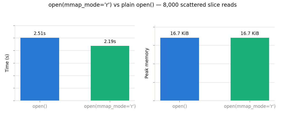
Across 8,000 scattered slice reads, mmap_mode="r" was ~1.2x faster. The higher peak on the mmap side is an accounting artifact, not extra memory: RSS charges the mapped pages the process touched, which are the same page-cache pages the plain-open() path reads through — just billed to the kernel there.
A single warm-cache process, as benchmarked here, is actually the worst case for showing mmap off — the payoff multiplies with several readers on the same file, which is the next tip.
Benchmark for this tip: tip_06_mmap_read.py
Many readers on one file? mmap in every one of them
When several processes read the same blosc2 file concurrently, open it with mmap_mode="r" in each reader. Every regular-I/O access pays a syscall plus a copy from the OS page cache into private buffers, and that per-access overhead compounds under kernel contention — while mmap readers all go straight to a single, shared set of mapped pages. So the speedup grows with the number of readers, and physical memory stays at roughly one copy of the file no matter how many readers attach.
# Avoid: each reader process pays syscalls + private buffer copies
arr = blosc2.open(path)  # reader 1..N

# Prefer: all readers share one set of mapped pages
arr = blosc2.open(path, mmap_mode="r")  # reader 1..N
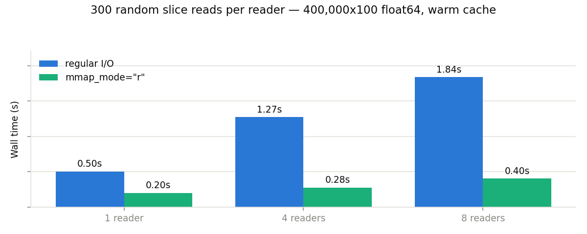
With 8 concurrent readers doing random slice reads over a 269 MB array, mmap was ~1.1x faster in wall time and used ~5% less total CPU; with one reader the two are level. Don’t be alarmed if mmap readers look heavier in RSS — each process charges the shared mapped pages it touched, but they exist once physically; per-process private memory is identical in both modes. The full discussion, including the measurement table, is in the Sharing containers across processes guide’s colophon; see that guide too for the multi-reader/NFS/Windows caveats.
That margin was much wider before C-Blosc2 3.3.1, which stopped reopening the frame file on every chunk access: the regular path caught up, mmap did not regress.
Benchmark for this tip: tip_10_mmap_many_readers.py
Use .b2z to group related data into one memory-mapped file
.b2z packs related data — a CTable’s columns and indexes, hierarchies of arrays, or both — into a single-file container that blosc2 reads in place: opened read-only, nothing is ever unpacked, and with mmap_mode="r" every member is memory-mapped at its offset inside the container. Beyond the convenience of one file to copy or archive, this buys you:
mmap out of the box — one mapping of one file covers the whole dataset, and the OS shares its pages across every reader process.
One file open instead of hundreds — a wide
.b2ddirectory can hold 100+ leaf files, each costing an open/stat metadata round-trip; on network filesystems or with cold caches, that latency dominates.Atomic replacement —
to_b2z()swaps the file atomically, so readers always see the complete old dataset or the complete new one, never a mix; a directory of files can’t guarantee that.No per-file allocation slack — many small leaves each round up to a filesystem block in a
.b2d; packed members don’t, which can shrink wide datasets considerably.Layout locality — members sit contiguously in one file, so full scans read sequentially instead of seeking across scattered files.
Don’t treat it as an archive to extract before use:
# Avoid: unpacking first — extra time and a second copy on disk
with zipfile.ZipFile("data.b2z") as z:
    z.extractall("data.b2d")
t = blosc2.open("data.b2d")

# Prefer: one open, one mapping, straight from the container
t = blosc2.open("data.b2z", mmap_mode="r")
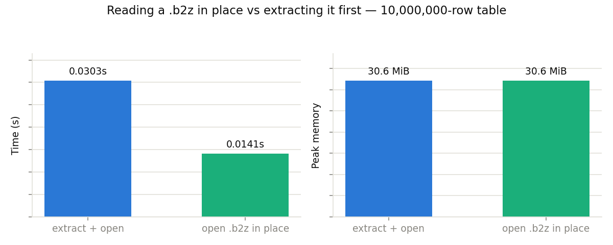
On a 10M-row table, opening in place and summing a column was ~3.4x faster than extract-then-open — both sides mmap_mode="r", so the only difference is the unpacking — at identical peak memory, and it leaves no unpacked copy behind. (This is one-shot filesystem work, measured with a single call, so the ratio varies with the filesystem and cache state.) The multi-reader advantages are the same as in the memory-map tip above, only with a single mapping serving the whole dataset.
One asymmetry to keep in mind: .b2z is optimized for reading, while a writable .b2z is staged in a temporary directory and rezipped on close — for write-heavy workloads, build the table as .b2d and pack it with to_b2z() when it’s ready to publish.
Benchmark for this tip: tip_09_b2z_read_in_place.py
Skip constraint checks in extend() with validate=False
You can pass a NDArray directly as a column value to CTable.extend(): both the write and the constraint validation happen chunk by chunk, so the array is never fully decompressed — it goes from compressed source to compressed column with only O(chunk) extra memory. Columns with no declared constraints skip validation automatically.
But for a column that does declare constraints (ge=, max_length=, …), validation still has to decompress and check every chunk; if you already know the data is valid, validate=False skips that pass.
# Default: every chunk is decompressed once to check declared constraints
t.extend({"val": src})

# Prefer, for known-good data: skip the constraint checks entirely
t.extend({"val": src}, validate=False)
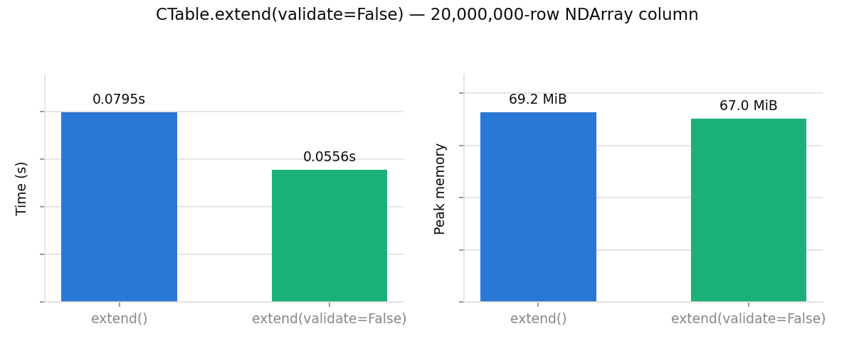
Extending a table with a 20M-row NDArray column carrying a ge=0 constraint, validate=False was ~1.4x faster; peak memory was within ~10%, since validation is chunk-wise anyway.
Benchmark for this tip: tip_07_chunked_writes.py